
Page 40 - IJOCTA-15-4
P. 40
Kazemi et al. / IJOCTA, Vol.15, No.4, pp.578-593 (2025)
for the components of the gradient ∂I and ∂I us- details. We do this by adding a scaled ver-
∂x ∂y
ing central difference approximations are done as sion of the tension field back to the origi-
11
follows : nal pixel image:
∂I I(x + 1, y) − I(x − 1, y)
≈ , I sharp = I + cτ(I), (13)
∂x 2
∂I I(x, y + 1) − I(x, y − 1)
≈ . (8) where c > 0 controls the intensity of the
∂y 2 sharpening effect. 15
3. Image smoothing: Although the ten-
These derivative approximations can be expressed sion field itself is noise-sensitive, its neg-
as convolution kernels in the filter form as: ative counterpart can be employed for
smoothing by simply subtracting the
−1 0 1 high-frequency components:
∂I 1
= −1 0 1 , (9)
∂x 2
−1 0 1 I smooth = I − cτ(I). (14)
and: However, this is less common than other
smoothing techniques (e.g., Gaussian fil-
tering) due to potential artifacts. 15
−1 −1 −1
∂I 1 4 Texture analysis: Breaks down an im-
= 0 0 0 . (10)
∂y 2 age into low-frequency and high-frequency
1 1 1
components that can be found useful for
Similarly, the Laplacian ∆I is approximated by: texture pattern analysis. By analyzing
how these components are spatially ar-
ranged/distributed, textures can be clas-
∆I ≈I(x + 1, y) + I(x − 1, y) + I(x, y + 1) sified or even material properties can be
+ I(x, y − 1) − 4I(x, y), (11) identified. 16
5 Image segmentation: The tension fields
accentuate areas of rapid intensity change,
for more details, see. 11,12 Using (7) and (11), serving as antecedent seeds for segmen-
the filter associated with the tension field τ(I) is tation algorithms, for example, region-
given by: growing or level-set methods. The
boundaries are usually aligned with ob-
0 1 0 ject boundaries or different parts in the
τ(I) = 1 −4 1 . (12) image. 17
0 1 0
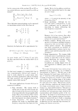
The tension field operator has a variety of ap-
plications in image processing, one of which is
As this kernel consists of a tension field that is
demonstrated in Figure 1. The left part of the
very computationally efficient and compact, it
figure illustrates the input image, which is the im-
may be easily adapted in a great many other
age of “Lena”one of the most popular references
image processing applications without sacrificing
in image processing as it consists of many details
the basic geometric and analytical idea of the and textures. The resulting image of the tension
original tension field concept. 13
field as an operator to the input image is shown in
the right part of the figure. This process, known
The major applications of tension field can be as edge detection, computes the tension field of
mentioned as follows:
the image, accentuating areas of rapid intensity
1. Edge detection: The tension field is change (e.g., edges and boundaries). This gives an
widely used in edge detection because the output which retains these characteristics (while
edge indicates where the second derivative smoothing out homogeneous areas), showing the
of an image intensity changes significantly. representation and extraction power of the ten-
Edges reflect zero-crossings of this tension sion field on the image of its interesting structural
field (useful for detecting the discontinu- information. Such examples showcase how func-
ities that separate two objects/regions). 14 tional the tension field can be both in enhancing
2. Image sharpening: The tension field as well as analyzing the image, thus serving as
sharpens the image by amplifying high- an efficiency tool for tasks like edge detection, de-
frequency components like edges and finer noising, and feature extraction.
582