Page 41 - IJOCTA-15-4

Nonlinear image processing with α-Tension field: A geometric approach

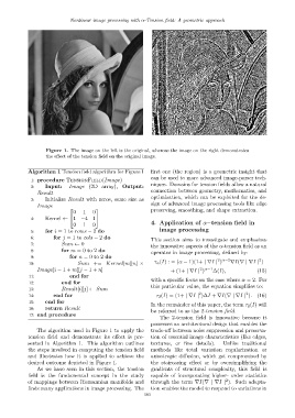
Figure 1. The image on the left is the original, whereas the image on the right demonstrates
the effect of the tension field on the original image.

Algorithm 1 Tension field algorithm for Figure 1 first one (the region) is a geometric insight that
can be used to more advanced image-parser tech-
1: procedure TensionField(Image)
niques. Domains for tension fields allow a natural
2: Input: Image (2D array), Output:
connection between geometry, mathematics, and
Result
optimization, which can be exploited for the de-
3: Initialize Result with zeros, same size as
sign of advanced image processing tools like edge
Image
  preserving, smoothing, and shape extraction.
0 1 0
4: Kernel ← 1 −4 1 

0 1 0 4. Application of α−tension field in
5: for i = 1 to rows − 2 do image processing
6: for j = 1 to cols − 2 do This section aims to investigate and emphasizes
7: Sum ← 0
the innovative aspects of the α-tension field as an
8: for m = 0 to 2 do
operator in image processing, defined by:
9: for n = 0 to 2 do 2 α−2 2
10: Sum += Kernel[m][n] × τ α (I) : = (α − 1)(1+ | ∇I | ) ∇I(∇ | ∇I | )
2 α−1
Image[i − 1 + m][j − 1 + n] + (1+ | ∇I | ) ∆(I), (15)
11: end for
with a specific focus on the case where α = 2. For
12: end for
this particular value, the equation simplifies to:
13: Result[i][j] ← Sum
2
2
14: end for τ 2 (I) = (1+ | ∇I | )∆I + ∇I(∇ | ∇I | ). (16)
15: end for In the remainder of this paper, the term τ 2 (I) will
16: return Result be referred to as the 2-tension field.
17: end procedure
The 2-tension field is innovative because it
possesses an architectural design that enables the
The algorithm used in Figure 1 to apply the trade-off between noise suppression and preserva-
tension field and demonstrate its effect is pre- tion of essential image characteristics (like edges,
sented in Algorithm 1. This algorithm outlines textures, or fine details). Unlike traditional
the steps involved in computing the tension field methods like total variation regularization or
and illustrates how it is applied to achieve the anisotropic diffusion, which get compromised by
desired outcome depicted in Figure 1. the staircasing effect or by oversimplifying the
As we have seen in this section, the tension gradients of structural complexity, this field is
field is the fundamental concept in the study capable of incorporating higher- order statistics
2
of mappings between Riemannian manifolds and through the term ∇I(∇ | ∇I | ). Such adapta-
finds many applications in image processing. The tion enables the model to respond to variations in
583