Page 130 - IJPS-11-4

International Journal of
Population Studies Environmental impact on Ukraine’s quality of life

2.3. Operationalization of variables Y = 11,153 − 0.005GRP + 0.004FDIR + 0.315PolAir +
t
t−1
t
t
Precise measures and operationalization of variables 0.893PolWater − 0.078Env + 0.017Health + 0.012 (II)
t
t
t
were employed to comprehensively analyze the factors To ensure the robustness of the regression analysis,
influencing mortality rates in the Carpathian region. a series of diagnostic tests were conducted to address
The dependent variable, “mortality rate,” represents the potential statistical issues. Autocorrelation was evaluated
number of deaths per 1,000 individuals, calculated as the using the Durbin–Watson statistic, which yielded values
median rate across the region’s four constituent oblasts: within acceptable ranges, indicating no significant
Zakarpattia, Ivano-Frankivsk, Lviv, and Chernivtsi. This autocorrelation in the residuals. Heteroscedasticity
measure provides a standardized and reliable indicator of was tested using the Breusch–Pagan test, revealing no
public health trends over the study period.
significant violations of homoscedasticity. This confirmed
Independent variables were carefully chosen to capture that the variance of residuals remains consistent across
the socioeconomic and environmental dimensions observations, satisfying one of the key assumptions of the
influencing mortality. GRP per capita serves as a proxy for OLS method.
regional economic prosperity, representing total economic
output divided by the population. This variable highlights The normality of residuals was assessed through graphical
the overall economic welfare of the region and its potential methods, such as Q-Q plots and the Shapiro–Wilk test. Both
impact on health outcomes. FDI, measured with a 1-year approaches confirmed that residuals align with normal
lag, reflects external economic activities and the possible distribution assumptions, ensuring the validity of statistical
introduction of industrial or polluting activities. The inferences drawn from the model. A correlation matrix was
lagged values allow for the time required for investments constructed to address potential multicollinearity (Table 2).
to impact the region’s socioeconomic and environmental None of the correlations between independent variables
dynamics. exceeded the critical threshold of 0.8, indicating no severe
multicollinearity issues.
Environmental indicators include emissions of air
pollutants (PolAir) and the discharge of contaminated
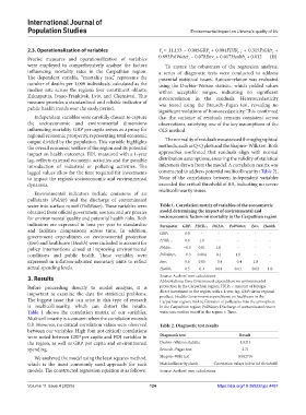
water into surface runoff (PolWater). These variables were Table 1. Correlation matrix of variables of the econometric
obtained from official government sources and are proxies model determining the impact of environmental and
for environmental quality and potential health risks. Both socioeconomic factors on mortality in the Carpathian region
indicators are expressed in tons per year to standardize Parameter GRPt FDIRt−1 PolAirt PolWatert Envt Healtht
and facilitate comparisons across time. In addition, 1.0 - - - - -
government expenditures on environmental protection GRPt
(Env) and healthcare (Health) were included to account for FDIRt−1 0.6 1.0 - - - -
policy interventions aimed at improving environmental PolAirt −0.3 0.01 1.0 - - -
conditions and public health. These variables were PolWatert −0.3 0.004 0.1 1.0 - -
expressed in inflation-adjusted monetary units to reflect Envt 0.6 0.05 −0.4 −0.4 1.0 -
actual spending levels. Healtht 0.5 0.3 0.01 0.01 0.02 1.0

3. Results Source: Authors’ own calculations.
Abbreviations: Envt: Government expenditure on environmental
Before proceeding directly to model analysis, it is protection in the Carpathian region; FDIRt−1: Amount of foreign
important to examine the data for statistical problems. direct investment in the region, with a 1-year lag; GRP: Gross regional
product; Health: Government expenditures on healthcare in the
The biggest issue that can arise in this type of research Carpathian region; PolAirt: Emission of pollutants into the atmosphere
is multicollinearity, which can distort the results. in the Carpathian region; PolWatert: Discharge of contaminated return
Table 1 shows the correlation matrix of our variables. water into surface runoff in the region; t: Time.
Multicollinearity is a concern when the correlation exceeds
0.8. However, no critical correlation values were observed Table 2. Diagnostic test results
between our variables. High (but not critical) correlations
were noted between GRP per capita and FDI variables in Diagnostic test Result
the region, as well as GRP per capita and environmental Durbin–Watson statistic 1.8314
spending. Breusch–Pagan test 2.71
We analyzed the model using the least squares method, Shapiro–Wilk test 0.982776
which is the most commonly used approach for such Multicollinearity check Correlation values below 0.8 threshold
models. The constructed regression equation is as follows: Source: Authors’ own calculations.

Volume 11 Issue 4 (2025) 124 https://doi.org/10.36922/ijps.4487