Page 10 - IJPS-2-1

Nonparametric graduation techniques as a common framework for the description of demographic patterns

A model with two versions capturing both the classical and the distorted fertility pattern was pro-
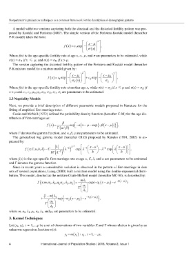
posed by Kostaki and Peristera (2007). The simple version of the Peristera-Kostaki model (hereafter
P-K model) takes the form:
  x µ  − 2 
f ( ) x = c 1 exp    σ ( ) x    ,  − 
   
Where f(x) is the age-specific fertility rate at age x, c 1, µ, and σ are parameters to be estimated, while
σ(x) = σ 11 if x ≤ µ, and σ(x) = σ 12 if x > µ.
The version capturing the distorted fertility pattern of the Peristera and Kostaki model (hereafter
P-K mixture model) is a mixture model given by:
  x µ 2    x µ  −  − 2 
f ( ) x = c exp   1   − + c exp   2  , −
 1   σ 1 ( ) x    2   σ 2  
   
Where f(x) is the age-specific fertility rate at mother age x, while σ(x) = σ 11 if x ≤ µ and σ(x) = σ 12 if
x > µ and c 1, c 2, µ 1, µ 2, σ 11, σ 12, σ 11, σ 2 are parameters to be estimated.

2.3 Nuptiality Models

Next, we provide a brief description of different parametric models proposed in literature for the
fitting of empirical first-marriage rates.
Coale and McNeil (1972) defined the probability density function (hereafter C-M) for the age dis-
tribution of first-marriages as:
β
f ( ) x = exp  ( ax µ − − exp − { β (x µ − )}) ,  −
Γ ( /a β )  
where Γ denotes the gamma function, and α, β, μ are parameters to be estimated.

The generalized log gamma model (hereafter GLG) proposed by Kaneko (1991, 2003) is ex-
pressed by:
λ λ − 2  1 xu  −  xu   − 
2
−
=
λ
f ( ; , , ,xC u b λ ) C ( ) ( ) exp λ  −  b  − λ − 2 exp λ   b      ,
−
2
bΓ λ      
where f(x) is the age-specific first marriage rate at age x, C, λ, and u are parameters to be estimated
and Γ denotes the gamma function.
Since in recent years a considerable variation is observed in the pattern of first-marriage in data
sets of several populations, Liang (2000) built a mixture model using the double-exponential distri-
bution. This model, denoted as the mixture Coale-McNeil model (hereafter MC-M), is described by:
mλ − (x µ − )
−
−
,
( ; , m α λ µα
f x 1 , , 1, 2 ,λ µ 2 ) = 1 exp( α 1 (x µ − 1 ) e 1 λ 1 )
2
1
Γ   α  1 
 λ 1 
(1 m λ )
−
) 2
+ exp α ( − 2 (x µ − 2 ) e − 2 λ (x µ − 2 ) ,
−
Γ   α  λ 2 
2 

where m, α 1, λ 1, μ 1, α 2, λ 2, and μ 1 are parameters to be estimated.
3. Kernel Techniques
Let (x i, y i), i = 1,…,p be a set of observations of two variables X and Y whose relation is given by an
unknown regression function m(x):
( ) ε+
y = mx , i = 1, , ,p
i i i
4 International Journal of Population Studies | 2016, Volume 2, Issue 1