Page 9 - IJPS-2-1

Anastasia Kostaki, Javier M. Moguerza, Alberto Olivares and Stelios Psarakis

model and the most widely used since 1980 is the one proposed by Heligman and Pollard (1980).
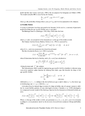
This model (hereafter HP) is described by the formula,
q x = A (xB+ ) C + De − ( (lnE x− ln )F 2 + GH ,
x
p
x
where q x is the probability of dying within a year, p x=1–q x, and A to H are parameters to be estimated.
2.2 Fertility Models

A variety of alternative have been proposed in the literature. In this section, a summary of parametric
models for fitting the age-specific fertility curve is provided.
The Hadwiger function (Hadwiger, 1940; Gilje, 1969) takes the form:
3
ab c 2  2 c x  


f ( ) x =  exp −  b  + − 2   ,
x
c    x c 
where a, b, and c are parameters to be estimated and x is the age of the mother at birth.
The Gamma function (Hoem, Madsen, Nielsen et al., 1981) is expressed by:
1 b− 1
f ( ) x = R (xd− ) exp ( ( {− xd− / c ))} , forx > d
Γ ( ) bc b
where R, b, c, and d are parameters that should be estimated.
The Beta function by Hoem et al. (1981) is given by:
Γ ( A B+ ) − ( AB ) 1 A− 1 B− 1
+−
x β ,
−
f ( ) x = R (βα ) (x α ) (β − ) x , for α <<
−
B
A Γ
Γ ( ) ( )
where R determines the level of fertility, and A, B, α, and β are calculated as:
(ν  α − )(β − ) v β  ν − ν α −
B = −  1  and A = B ,
−
−
 τ 2  β α βν
2
v being the mean and τ the variance.
The Schmertmann (2003) model for representing age-specific fertility schedules is obtained using
a piecewise quadratic spline function by defining three index ages that describe the shape of the
age-specific fertility:
 4 2
R* ∑ θ  (x t ) , α − x β ≤≤
f(x) =  k= 0 k k +

 0, otherwise ,
with Knots t 0 < t 1 < …< t 4 falling in the interval between ages α and β, where t 0 = α, (the lowest age
of childbearing) and (t t− k ) ≡ * MAX [0, x t− k ] .
A deviation from its classical shape in terms of a bulge in fertility rates of younger women is exhib-
ited by recent fertility patterns of some developed countries. Chandola et al. (1999) developed a
two-component mixture model of the Hadwiger function for the description of distorted fertility pat-
terns:

b  1  c 1  3/2     c x    b  2  c 2  3/2    c x   
−
f ( ) x = am    exp −   b 1  2 1 + − 2   + (1 m )    exp −  b 2  2 2 + − 2   ,
c 1   x     x c 1     c 2   x    x c 2    
Where x is the age of the mother at birth, and parameters m, α, b 1, c 1, b 2, and c 2 are to be estimated,
resulting in a seven parameter model by the inclusion of an additional parameter (Ortega and Kohler,
2000).

International Journal of Population Studies | 2016, Volume 2, Issue 1 3