Page 100 - AIH-1-3

Artificial Intelligence in Health ISM: A new multi-view space-learning model

Output: Factoring matrices W  nd e , H  dd e where d is the
e
embedding dimension, and is the sum of the number of columns in all
views and d vm d the matrix of concatenated views X.
v

1: Concatenate the m views: X X , , X , X nd ;

m
1

2: Factorize X using NMF with d components:
e

XWH T E W ,  nd e , H  dd e , E  nd ;

(ii) Unit 2: Parsimonization
The initial degree of sparsity of H is crucial to prevent
the embedding dimensions from being overly distorted
between the different views during the embedding process,
as will be seen in the next section. This is achieved by
applying a hard threshold to each column of the H matrix.
The threshold is based on the reciprocal of the Herfindahl-
Hirschman index (HHI), which provides an estimate of
30
the number of non-negligible values in a non-negative
vector.
For columns with strongly positively skewed values,
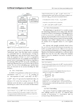
Figure 2. Training of the integrated sources model the use of the L2 norm for the estimate’s denominator can
lead to excessively sparse factors, which in turn can lead
units enable the discovery of the latent space within an to an overly large approximation error during embedding.
“embedding” space. Once the latent space is identified, Therefore, the estimate is multiplied by a coefficient whose
it is assimilated with the embedding space. During the default value was set at 0.8, after testing with simulated
fifth “straightening” unit, the latent space remains fixed, datasets using the simulation framework described in
while the sequence of Units 3, 4, and 2 is repeated to Fogel et al. 31
further parsimonize the view-mapping until the degree of
sparsity remains unchanged. The theoretical foundations Unit 2. Parsimonization
of combining NMF and NTF during the embedding and Input: Factoring matrix
latent space discovery steps are discussed at the end of this dd e

section. The sizes of the embedding space and the latent Output: Parsimonized factoring matrix H  (since the initial H is
space are discussed in the section describing the third not used outside parsimonization, we use the same symbol for the sake
of simplicity).
workflow.
1: for each component h of H do
k
(i) Unit 1: Initialization 2: Calculate the reciprocal of the Herfindahl-Hirschman Index to
An NMF is first performed on the matrix X of the m estimate the number of non-negligible entries in h : k
concatenated views X , 1 ≤ v ≤ m, resulting in id , 2 h 2
hi k
v k1 ;

the decomposition: XWH T E W ,  nd e , H  dd e , k id , 2 h k2 2
hi k

E nd where W represents the transformed data, the 3: Enforce sparsity on hk using hard thresholding:
columns of H contain the loadings of the d vm d If rank (h [i, k]) < τ × λ then set h [i, k] = 0 where λ is a sparsity
k
parameter (0 < λ < 1, the default value λ = 0.8 was chosen as it led in
v

attributes across all views on each component, d is the many trials to better results than the original index τ , which may be
e
k
embedding size, and n is the total number of observations. a too strict filter);
4: end for
Unit 1. Initialization
(iii) Unit 3: Embedding

Input: m views {X , , X }, X  nd v where n is the number of rows The matrices W and H are further updated along each
1 m v

common to all views and d is the number of columns in the v view view, yielding matrices W  nd e of common shape
th
v
v

(it is assumed for each column that its values lie between 0 and 1 after (number of observations n × factorization rank d )
normalization by the maximum row value). corresponding to the transformed views. e
Volume 1 Issue 3 (2024) 94 doi: 10.36922/aih.3427