Page 101 - AIH-1-3

Artificial Intelligence in Health ISM: A new multi-view space-learning model

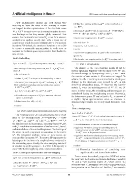
NMF multiplicative updates are used during view dd e as the concatenation of

matching to leave the zeros in the primary H matrix 1: Define view-mapping matrix H 
v
dd e
unchanged. Further optimizations of the simplicial cones H  ;
v
H  d v d e for each view v are therefore limited to the non- 2: Factorize using NTF with d components: = W*⨂H*⨂Q*+ ε
i
v

e

zero loadings so that they remain tightly connected. This where W  * nd l , H  * dd l , Q  * md l , nd m ;
e

ensures that the transformed views W , v ≤ m, form a tensor. 3: Update view-mapping matrix H  : H ← HH*;

v
dd l
Multiplicative updates usually start with a linear rate of
convergence, which becomes sublinear after a few hundred 4: for each view v do
iterations. By default, the number of iterations is set to 200 5: Update H : H ← H ∘ Q* [v, :];
32
v
v
v
to ensure a reasonable approximation to each view, as 6 end for
required for the latent space representation described in the dd l as the concatenation of

next section. 7: Update view-mapping matrix H 
updated H ; v
Unit 3. Embedding dd l by applying Unit 2;

8: Parsimonize view-mapping matrix H 

Input: m views {X , …, X } and factoring matrices W  nd e , H  dd e . (v) Unit 5: Straightening
1 m
v

Output: view-specific factoring matrices W  nd e , H  dd e and The sparsity of the view-mapping matrix H can be

v

v
tensor . further optimized together with the meta-scores W* and
1: for each view v do the view-loadings Q* by repeating Units 3, 4, and 2 until
the number of zero entries in H remains unchanged. To
v
2: Define H  dd e as the part of H corresponding to view v;
v achieve this, the embedding is restricted to the latent space

v
3: Factorize X into view-specific W  nd e and using H  dd e defined by the simplicial cone formed by H*. In this
v
v

v
NMF multiplicative updating rules and initialization matrices simplified embedding space, H* becomes the identity
W  nd e , H  v dd e : matrix I when the updating process of W*, H*, and Q*
v

d l
v

X W H v T E W , v  nd e , H  v dd e , E  nd v ; starts. In other words, the embedding and latent spaces are
v
v

v
v

4: Normalize each component of W by its maximum value and assimilated during the straightening process. Optionally,
for faster convergence, H* can be fixed to I , at the cost of
v
update H accordingly; d l
v a slightly higher approximation error, as observed in

5: Define tensor slice:  :,:,v W ; simulated experiments, due to only small deviations from
v
I .
6: end for d l
Unit 5. Straightening
(iv) Unit 4: Latent space representation and view-mapping
Input: X, , H, W*, H*, Q*.
The resulting tensor is analyzed using NTF, which
leads to the decomposition: =W*⨂H*⨂Q*+ε where Output: NTF factors W*, H*, Q* and updated view-mapping matrix H.
*

*

m
*
W  nd l , H  d e d l , Q  md l ,  nd e , and d is 1: H = I Set where d is the size of the latent space;
*
l
d l
i

the dimension of the latent space. The components W*, H*, 2: do until the number of 0-entries in H remains unchanged
and Q* enable the reconstruction of the horizontal, lateral, 3: Apply Unit 3 to embed X using the embedding size d =d,
and frontal slices of the embedding tensor. The loadings of initialization matrices W  nd l and view-mapping matrix
e
l

*

the views on each component are contained in the matrix H  dd l found in the previous iteration;

Q*. The integrated multiple views, or meta-scores, are 4: Apply Unit 4 to factorize and update the view-mapping matrix
contained in the matrix W*. The matrix H* represents the H  dd l , using embedding size d =d, initialization matrices W*,

l
e
latent space in the form of a simplicial cone contained in H*, Q* obtained in the previous iteration and fixed H = I ;
*
the embedding space. Finally, the view-mapping matrix H d l
is updated by applying steps 3 – 8 of Unit 4. Its sparsity is 5: end for
ensured by further applying Unit 2 (parsimonization). (vi) Theoretical foundations of combining non-
Unit 4. Latent space representation and view‑mapping negative matrix and tensor factorization
From a more theoretical perspective, NMF estimates,
v
Input: view-specific factoring matrices H  dd e and tensor .
v for each view, the transformed data in the form of a matrix
W and a view-mapping matrix H , which allows the

*
e
Output: NTF factors W  * nd l , H  * dd l , Q  md l and reconstruction of the original view. Following a geometrical
v
v

view-mapping matrix H  dd l . interpretation from Donoho and Stodden, we consider

33
Volume 1 Issue 3 (2024) 95 doi: 10.36922/aih.3427