Page 80 - AJWEP-22-5

Jun, et al.

The “MSE increase” and “standard deviation (Std)” implementations. The computational framework utilized
values for each parameter are presented in Table 3. Python and the Keras deep learning framework, with
29
28
“MSE increase” refers to the average increase in the GPU acceleration enabled for training.
model’s prediction error, compared to the original
data, after shuffling a specific feature. “Std” indicates 4.2. Model settings
the variability in the MSE increase across multiple The neural network comprises an LSTM layer for
shuffling repetitions. A smaller standard deviation temporal feature extraction and a dense layer for
suggests a more stable and reliable assessment of regression output. Critical hyperparameters, including
30
feature importance, while a larger standard deviation the number of LSTM units and the learning rate, were
indicates greater uncertainty in the evaluation due to optimized using an evolutionary approach. MSE
32
31
varying impacts across shuffles. was employed as the loss metric to evaluate regression
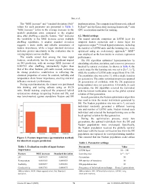
The results reveal that among the four input performance.
features, conductivity has the most significant impact The DE algorithm optimized hyperparameters by
on DO prediction, with an average MSE increase of simulating selection, mutation, and crossover processes
0.005783 after shuffling, substantially higher than inspired by natural evolution. As shown in Table 4, the
that of the other features. pH ranks second, indicating search range for the learning rate was set to [1e , 1e ],
−4
−2
its strong predictive contribution in reflecting the while the number of LSTM units ranged from 10 to 100.
chemical properties of water. In contrast, turbidity and The population size was set to 15, with a single iteration
temperature show lower importance, exerting minimal per generation. The entire optimization process spanned
influence on model performance. 20 generations of evolution, with the DE population
During experimentation, the dataset was partitioned being updated once per generation. Ultimately, in each
into training and testing subsets using an 80:20 generation, the DE algorithm selected the individual
ratio. Model training employed the proposed hybrid with the lowest verification loss as the global optimal
optimization strategy integrating Nadam and DE, and solution of that generation.
was benchmarked against standalone Nadam and DE In each generation, the Nadam optimization algorithm
was used to train the model individuals generated by
DE. The Nadam population size was set to 5, and each
individual randomly generated a different learning
rate and number of LSTM units. Nadam trained each
individual and selected the best-performing one as the
local optimal solution for that generation.
During the optimization process, every two
generations, the optimal individuals from the DE and
Nadam populations were exchanged. Specifically,
the Nadam population received the globally optimal
individual with the lowest verification loss from the DE
population and replaced its worst-performing member.
Figure 3. Feature importance (permutation method) This ensured that the Nadam population could utilize
for dissolved oxygen prediction
Table 4. Parameter settings
Table 3. Evaluation results of input feature Parametric Value
importance LSTM layer 10 – 100

Feature MSE increase Standard deviation Learning rate 1e – 1e −2
−4
pH 0.003135 0.000362 Generation 30
Temperature 0.001345 0.000523 DE number of iterations 10
Turbidity 0.000697 0.001291 DE population size 15
Conductivity 0.005783 0.000875 Frequency of information exchange Every 2 generations
Abbreviations: MSE: Mean squared error; Std: Standard Abbreviations: DE: Differential evolution; LSTM: Long
deviation. short-term memory.

Volume 22 Issue 5 (2025) 74 doi: 10.36922/AJWEP025210165