Page 78 - AJWEP-22-5

Jun, et al.

terminates, and the global optimal parameter θ* is ' XX min
−
output for model deployment. X = X max − X min (XXIV)
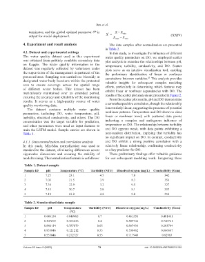
4. Experiment and result analysis The data samples after normalization are presented
in Table 2.
4.1. Dataset and experimental settings In this study, to investigate the influence of different
The water quality dataset used in this experiment water quality parameters on DO, we employed scatter
was obtained from publicly available secondary data plot analysis to examine the relationships between pH,
on Kaggle. The water quality information in the temperature, turbidity, conductivity, and DO. Scatter
dataset was regularly collected by volunteers under plots serve as an intuitive visualization tool, enabling
the supervision of the management department of the the preliminary identification of linear or nonlinear
protected area. Sampling was carried out biweekly at associations between variables. This analysis provides
25
designated water body locations within the protected valuable insights for subsequent complex modeling
area to ensure coverage across the spatial range efforts, particularly in determining which features may
of different water bodies. This dataset has been
meticulously maintained over an extended period, exhibit linear or nonlinear dependencies with DO. The
ensuring the accuracy and reliability of the monitoring results of the scatter plot analysis are presented in Figure 2.
results. It serves as a high-quality source of water From the scatter plot results, pH and DO demonstrate
quality monitoring data. a somewhat positive correlation, though the relationship
The dataset contains multiple water quality is not strictly linear, suggesting the presence of potential
parameters, including DO, water temperature, pH, nonlinear patterns. Temperature and DO show no clear
turbidity, electrical conductivity, and others. The DO linear or nonlinear trend, with scattered data points
concentration was the target variable for prediction, indicating a complex and ambiguous influence of
and other parameters were used as input features to temperature on DO. The relationship between turbidity
train the LSTM model. Sample entries are shown in and DO appears weak, with data points exhibiting a
Table 1. near-random distribution, implying that turbidity has
no significant impact on DO. In contrast, conductivity
4.1.1. Data normalization and correlation analysis and DO exhibit a strong positive correlation with a
In this study, Min-Max normalization was used to relatively linear relationship, confirming conductivity
standardize the dataset, eliminating differences across as a key predictor for DO.
eigenvalue dimensions and ensuring the stability of These preliminary findings offer valuable guidance
model training. The normalization formula is as follows: for our subsequent modeling work. Integrating these

Table 1. Dataset sample
Sample ID pH Temperature (°C) Turbidity (NTU) Dissolved oxygen (mg/L) Conductivity (S/cm)
1 7.25 23.1 4.5 7.8 342
2 7.03 21.5 3.9 8.3 356
3 7.38 22.9 3.2 9.5 327
4 7.45 20.7 3.8 8.1 352
5 7.19 21.2 4.2 8.8 350

Table 2. Standardized data sample
Sample ID pH Temperature Turbidity (NTU) Dissolved oxygen (mg/L) Conductivity (S/cm)
(°C)
1 0.646154 0.848485 0.7 0.461538 0.481481
2 0.307692 0.363636 0.4 0.589744 0.740741
3 0.846154 0.787879 0.05 0.897436 0.203704
4 0.953846 0.121212 0.35 0.538462 0.666667
5 0.553846 0.272727 0.55 0.717949 0.62963

Volume 22 Issue 5 (2025) 72 doi: 10.36922/AJWEP025210165