Page 87 - IJAMD-2-2

International Journal of AI for
Materials and Design Fruit image detection using AI

feature values into the same range. This prevents any single 2.3. Comparison of kernel functions
feature from having too much influence over the model’s The different kernel functions were benchmarked against
performance.
each other based on their performance in efficiently
2.2.2. Training the model classifying the fruits. This evaluation utilized several
performance metrics, including accuracy, precision, recall,
To train the model, the system splits the entire dataset into and F1 score, all derived from confusion matrix analyses.
two parts: One for training and one for testing. It used 70%
of the data in training the model and kept the other 30% 2.3.1. Confusion matrix method
to test the training efficiency. Then, the SVM model was
trained using the selected features. The study also used One of the most effective approaches for evaluating the
kernel functions to transform the feature space, which performance of the trained classification model is the
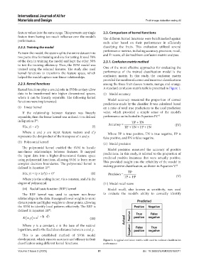
helped the model capture non-linear relationships. confusion matrix. In this study, the confusion matrix
provided the number of correct and incorrect classifications
2.2.3. Kernel functions among the three fruit classes: tomato, mango, and orange.

Kernel functions play a crucial role in SVMs as they allow A standard confusion matrix table is presented in Figure 1.
data to be transformed into higher dimensional spaces, (i) Model accuracy
where it can be linearly separable. The following kernel
functions were implemented: Model accuracy measured the proportion of correct
predictions made by the classifier. It was calculated based
(i) Linear kernel on a ratio of total true predictions to the total prediction
If the relationship between features was linearly value, which provided a simple sense of the model’s
separable, then the linear kernel was utilized. It is defined performance as indicated in Equation IV. 41
in Equation I : TP + TN
38
Accuracy = (IV)
K(x, y) = x y (I) TP + TN + FP + FN
T
Where x and y are input feature vectors and x y Where TP is true positive, TN is true negative, FP is
T
represents the dot product of the transpose of x and y. false positive, and FN is false negative.
(ii) Polynomial kernel (ii) Model precision
The polynomial kernel enabled the SVM to handle Model precision measured the accuracy of positive
non-linear relationships between features. It mapped predictions. In this study, it referred to the proportion of
the input data into a higher-dimensional feature space predicted positive instances that were actually positive.
using polynomial functions, allowing SVM to learn more This provided insight into the reliability of the model in
complex decision boundaries. The polynomial kernel is 42
defined in Equation II : making positive classification, as shown in Equation V.
39
K(x, y) = (γ × (x y) + r) d (II) Precision = TP (V)
T
Where γ is the scaling factor, r is a constant, and d is the TP + FP
degree of polynomial. (iii) Model recall score
(iii) Radial basis function (RBF) kernel Model recall, also known as sensitivity, was used
The RBF kernel was used to capture non-linear to evaluate the model’s ability to correctly identify
relationships in the data. It assigned lower weights to more
distant points and higher weights to closer points, allowing
the SVM to identify local patterns effectively. The RBF is
defined in Equation III :
40
K ( ,xy ) e= ( * x y )−γ − 2 (III)

Where γ is a constant, e is the base of the natural
logarithm, and is the Euclidean distance between x and y.
This is an established method of SVM model
development, which ensures accuracy and efficacy in fruit Figure 1. A typical confusion matrix table used to evaluate classification
classification using different kernel functions. performance

Volume 2 Issue 2 (2025) 81 doi: 10.36922/IJAMD025150011