Page 27 - IJOCTA-15-2

A. R´acz / IJOCTA, Vol.15, No.2, pp.215-224 (2025)
and waste costs (CW = 100, CC = 400) as
in the numerical example. Optimalon offered a
very short trial period, so only 10 test cases were
solved. The full data set can be found in Table
A1. in the Appendix.

Table 9 shows the ranking based on the num-
ber of cuts. There is not much difference in the
number of cuts. There are only a few cases where
there is a difference between the obtained plans,
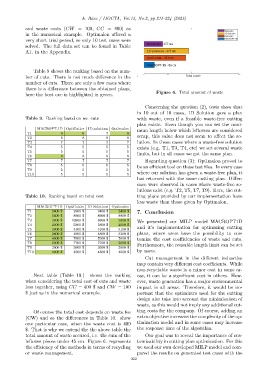
Figure 6. Total amount of waste
here the best one is highlighted in green.

Concerning the question (2), tests show that
in 10 out of 10 cases, 1D Solution gave a plan
Table 9. Ranking based on no. cuts with waste, even if a feasible waste-free cutting
plan exists. Even though you can set the mini-
MACROPT-1D OptiCutter 1D solutions Optimalon mum length below which leftovers are considered
T1 6 6 7 6
T2 8 8 8 8 scrap, this value does not seem to affect the so-
T3 7 7 7 7 lution. In those cases where a waste-free solution
T4 5 5 5 5 exists (e.g. T1, T3, T4, etc) we set several waste
T5 5 5 5 5 limits, but in all cases we got the same plan.
T6 6 8 8 8
T7 7 7 7 7 Regarding question (3): Optimalon proved to
T8 5 5 5 5 be an efficient tool on these test files. In every case
T9 5 5 5 5
T10 5 5 5 5 where our solution has given a waste-free plan, it
has returned with the same cutting plan. Differ-
ence were observed in cases where waste-free so-
lutions exist (e.g. T2, T5, T7, T9). Here, the cut-
Table 10. Ranking based on total cost ting plans provided by our implementation have
less waste than those given by Optimalon.
MACROPT-1D OptiCutter 1D Solutions Optimalon
T1 2400 $ 2900 $ 9400 $ 2400 $ 7. Conclusion
T2 5600 $ 8900 $ 8900 $ 8900 $
T3 2800 $ 10900 $ 6900 $ 2800 $ We presented our MILP model MACROPT1D
T4 2000 $ 5800 $ 5800 $ 2000 $
T5 3000 $ 3100 $ 3100 $ 3100 $ and it’s implementation for optimizing cutting
T6 2400 $ 4800 $ 4800 $ 3200 $ plans, where users have the possibility to cus-
T7 4600 $ 7600 $ 7600 $ 7600 $ tomize the cost coefficiencies of waste and cuts.
T8 2000 $ 7700 $ 7700 $ 2000 $ Furthermore, the reusable length limit can be set
T9 3600 $ 3600 $ 3600 $ 3600 $
T10 4000 $ 4500 $ 4500 $ 4500 $ by users.
Cut management in the different indusrties
may contain very different cost coefficients. While
non-recyclable waste is a minor cost in some ar-
Next table (Table 10.) shows the ranking eas, it can be a significant cost in others. How-
when considering the total cost of cuts and waste ever, waste generation has a major environmental
loss together, using CC = 400 $ and CW = 100 impact in all areas. Therefore, it would be im-
$ just as in the numerical example. portant that the optimizers used for the cutting
design also take into account the minimization of
waste, as this would not imply any additional cut-
Of course the total cost depends on waste fee ting costs for the company. Of course, adding an
(CW) and so the differences in Table 10. show extra objective increases the complexity of the op-
one particular case, when the waste cost is 400 timization model and in some cases may increase
$. That is why we extend the the above table the the response time of the algorithm.
total amount of waste accured, i.e. the sum of the Our goal was to reveal the importance of cus-
leftover pieces under 45 cm. Figure 6. represents tomizability in cutting plan optimization. For this
the efficiency of the methods in terms of recycling we used our own developed MILP model and com-
or waste management. pared the results on generated test cases with the
222