Page 22 - IJOCTA-15-2

A MILP model for one dimensional cutting stock problem with adjustable leftover threshold . . .
2.2. Minimization of cutting cost we need to introduce the definition of waste. Left-
over with a length that is below the user-defined
In this initial version of our model we consider
limit, LOl j < W is considered as waste. We also
the total cost of cuts as an objective (in (1)), sub-
introduced binary variables WL j , j = 1, . . . , n
ject to serving all orders. The objective function
to indicate whether the leftover are reusable or
1 defines the total cost of the cuts by counting
waste. Value of variable WL j should be deter-
them and multiplying with the user defined cut-
mined as follows:
ting cost, coeffitient CC.
The number of cuts is determined by the num- 0 if LOl j >= W,
ber of orders assigned to the bar as follows: WL j =
LOl j , else.
Number of cuts on bar B j is
Decision makers are also able to define the
m
 P
 i=1 x ij , if there is some leftover, waste cost: CW, that is the unit loss on waste.
Depending on their length, trim losses may be
P m
 x ij − 1, else.
i=1 added to the total cost.
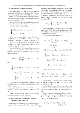
The new objective function is:
Where x ij binary variable denotes the assigne-
ment between orders and bars, so that x ij = 1, if n m
X X
the order O i is served by the bar B j , else x ij = 0. min CC · (x ij ) − 1 + Y L j
According to the notations in Table 1, binary j=1 i=1 (5)
variable Y L j determines whether there is a re- n
X
mainder on bar B j or not. + CW · WL j
The model allows the user to define a cutting j=1
fee CC parameter, that can be inserted into the with previously defined constraints (2) - (4):
objective function. So the model can be formu-
lated as follows: m
X
x ij r i + LOl j = l j j = 1, 2, . . . , n
n m i=1
X X
min CC · x ij − 1 + Y L j (1) LOlj
j=1 i=1 Y L j ≥ j = 1, 2, . . . , n
l j
st.
n
X
x ij = 1 i = 1, 2, . . . , m
m
X j=1
x ij r i + LOl j = l j j = 1, 2, . . . , n (2)
i=1 and extended with two more:
LOlj
Y L j ≥ j = 1, 2, . . . , n (3)
l j j = 1, 2, . . . , n (6)
LOl j − WL j ≤ M · Y R j
n
W −LOl j ≤ M ·(1−Y R j ) j = 1, 2, . . . , n. (7)
X
x ij = 1 i = 1, 2, . . . , m (4)
j=1
Where M is a constant that is large enough
Constraint (2) ensures that the length of a bar so that W − LOl j ≤ M and LOl j − WL j ≤ M,
should be equal to the leftover and the sum of the ∀j ∈ {1, 2, . . . , n}.
orders assigned to it. Constraints (6) and (7) are the regular for-
Constraint (3) sets the value of Y L j binary malization of if-then logical constraints (for more
variables to reflect the existense of leftover on bar details see 13 Chapter 9.1.) in the following con-
B j . tex:
Finally, constraint (4) ensures that, an order If the length of the leftover (LOl j ) is shorter
can only belong to exactly one bar. than the reuse limit (W), then it is a waste
WL j = LOl j , else there is no waste on bar B j
2.3. Extending the model with leftover , WL j = 0. In other words:
threshold and trim loss

In this version of our model, we extended the cost If LOl j < W, then WL j = LOL j ,
function with losses/penalties from waste. First, else WL l = 0.
217