Page 47 - IJOCTA-15-4

Nonlinear image processing with α-Tension field: A geometric approach
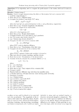
Algorithm 2 The algorithm used to compare the performance of the tension field and 2-tension in
Figure 2.
Require: Original image I
Ensure: Output images demonstrating the effects of the tension field and α-tension field
1: Load the original image I.
2: Store this as (a 1 ): Original image.
2
3: Compute the gradient magnitude |∇I| using:
2
2
|∇I| = (∂ x I) + (∂ y I) 2
where ∂ x I and ∂ y I are partial derivatives in the x- and y-directions, respectively.
4: Store this as (a 2 ): Gradient magnitude visualization.
5: Compute the output of the tension field:
τ(I) = ∆I

where ∆I is the Laplacian of I.
6: Store this as (b 1 ): Tension field output.
7: Compute Sobel-X (∂ x I) and Sobel-Y (∂ y I) gradients:
8: (b 2 ): Horizontal edge details (Sobel-X).
9: (c 1 ): Vertical edge details (Sobel-Y).
10: Compute the first term of the α-tension field:
2
T 1 = (1 + |∇I| )∆I
2
where |∇I| controls adaptive diffusion.
11: Store this as (c 2 ): Visualization of the first term.
12: Compute the second term of the α-tension field:
2
T 2 = ∇I · (∇|∇I| )
2
where ∇|∇I| captures higher-order gradient information.
13: This term detects corners, junctions, and fine details.
14: Store this as (d 1 ): Visualization of the second term.
15: Combine terms to compute the α-tension field for α = 2:

τ α (I) = T 1 + T 2
where:
2
16: T 1 = (1 + |∇I| )∆I,
2
17: T 2 = ∇I · (∇|∇I| ).
18: Store this as (d 2 ): Final output of the α-tension field.
19: Compare results:
20: Tension field (b 1 ): Efficient edge detection but amplifies noise.
21: α-Tension field (d 2 ): Retains structure while filtering noise effectively.
22: Summary of outputs:
23: (a 1 ): Original image.
2
24: (a 2 ): Gradient magnitude |∇I| .
25: (b 1 ): Tension field output.
26: (b 2 ): Sobel-X gradient.
27: (c 1 ): Sobel-Y gradient.
28: (c 2 ): First term of α-tension field.
29: (d 1 ): Second term of α-tension field.
30: (d 2 ): Final α-tension field output.

as edges, corners, and fine details to be conserved desirable in areas such as medical imaging or
and even accentuated. The magnitude of the 2- wherever structural integrity is important. The
tension field makes the algorithm highly flexible first term of this equation regulates the diffusion,
when it comes to more advanced functionalities, relying on the spatial change and suppression of
including denoising, edge-preserving, smoothing, diffusion in the regions of high gradients to pre-
and feature enhancement, all of which are highly serve the edges, while the second term keeps the
589