Page 49 - IJPS-3-2

Desta CG

Appendix B

1
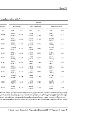
Parameter estimates for maternal productive work participation by the number of children and control variables

Exogenous probit Ivprobit

Variables Full sample Urban sub-sample Rural sub-sample Full sample Urban sub-sample Rural sub-sample

Coef. p>z Coef. p>z Coef. p>z Coef. p>z Coef. p>z Coef. p>z

0.0918 -0.2156 0.1568 0.1671 0.0304 0.8412
Number of children 0.070 0.061 0.004 0.418 0.113
(0.0321) (0.0452) (0.0425) (0.2031) (0.1549) 0.315 (0.1456)
0.0982 0.0352 0.0934 0.0745 0.0112 -0.0785
Average age of children 0.113 0.421 0.101 0.211 0.107 0.113
(0.0241) (0.0098) (0.0401) (0.0127) (0.0198) (0.0345)
0.1845 0.5145 0.1305 0.1562 0.3190 0.1052
Sex of household head 0.451 0.054 0.625 0.408 0.301 0.651
(0.1987) (0.1845) (0.3512) (0.2189) (0.3163) (0.4009)
-0.0107 0.0212 -0.826 -0.0564 -0.1151 -0.0777
Age of household head 0.201 0.213 0.071 0.215 0.412 0.137
(0.0074) (0.0151) (0.0321) (0.0170) (0.0338) (0.0307)
0.1342 0.2221 0.0997 0.1121 0.2241 0.1057
Participant’s age at first marriage 0.105 0.265 0.415 0.511 0.671 0.253
(0.0361) (0.0212) (0.0121) (0.0415) (0.0501) (0.0512)
0.0095 0.0886 -0.0213 0.0652 0.0757 0.0152
Years of schooling of the participant 0.524 0.111 0.671 0.214 0.201 0.221
(0.0555) (0.0346) (0.0358) (0.0398) (0.0322) (0.0333)
Contraceptive use (Yes=1, 0.1412 0.346 0.4141 0.208 0.1111 0.741 0.1127 0.581 0.4025 0.289 0.0120 0.888
Otherwise=0) (0.1042) (0.2112) (0.5242) (0.2020) (0.4240) (0.4151)

0.1919 0.7194 0.1145 0.2191 0.4171 0.1515
Loan receipt (Yes=1, Otherwise=0) 0.230 0.031 0.366 0.444 0.111 0.424
(0.1701) (0.1939) (0.1212) (0.0881) (0.2235) (0.2320)
Members other than parents engaged 0.3323 0.012 0.6652 0.051 0.2002 0.216 0.4097 0.143 0.6076 0.068 0.2451 0.019
in non-productive work (0.1545) (0.2145) (0.2525) (0.1818) (0.3041) (0.4041)

Members other than parents engaged -0.0989 0.601 0.4909 0.134 -0.5021 0.129 -0.0666 0.184 0.4098 0.113 -0.5142 0.101
in productive work (0.1801) (0.2554) (0.2444) (0.1965) (0.2828) (0.2099)

Mean hours of daily work by
0.3541
-0.0819
-0.2535
0.2514
-0.1452
-0.6852
household members (excluding (0.1745) 0.521 (0.2513) 0.125 (0.2242) 0.210 (0.2004) 0.241 (0.2156) 0.121 (0.2002) 0.127
parents)
0.0194 -0.6523 0.5262 0.0098 -0.8898 0.1104
Constant 0.699 0.214 0.115 0.721 0.235 0.546
(0.2524) (0.5124) (0.1426) (0.4251) (0.9859) (9445)
1 Covariates controlled. Because of the endogeneity of fertility to economic indicators, employing the ordinary least squares (OLS) estimator in which maternal labor market participation is regressed on the observed
number of children becomes misleading. To acknowledge this problem, the two stage instrumental variable was used. In the first stage, the observed number of children were regressed on sex composition of the first
two siblings borne to a woman (1=same sex; 0, Otherwise), plus other covariates controlled in the model. In the second stage, maternal labor supply was regressed on the predicted number of children (predicted in the
first stage) as the key independent variable of interest, plus the same variables control in the first stage. The idea is that sibling sex mix (the instrumental variable) determines the number of children exogenously (i.e.,
it has direct effect on the number of children, but no effect on maternal labor supply). For comparison purpose, both exogenous (exogenous probit) and endogenous models (ivprobit) were estimated. Standard errors
are reported in parentheses.

42 International Journal of Population Studies | 2017, Volume 3, Issue 2