Page 26 - IJPS-4-1

Transition to first marriage in China

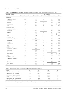
Table 4. Joint distribution (in percentage) of husband’s and wives’ education, overall and by marriage cohort (n=19,340).
Husband’s education Wife’s education
Primary school and below Junior middle High school College and more Total
All respondents
Primary school and below 22.6 4.7 0.8 0.1 28.1
Junior middle 14.4 16.8 3.9 0.7 35.7
High school 3.8 6.9 8.2 2.0 20.9
College and more 0.5 1.7 4.0 9.0 15.2
Total 41.4 30.1 16.9 11.7 100.0
1966–1979 (n=4,080)
Primary school and below 46.1 4.2 0.6 0.0 51
Junior middle 17.9 9.1 2.2 0.6 29.9
High school 5.4 4.0 2.9 0.7 13.0
College and more 1.1 1.5 2.1 1.4 6.2
Total 70.5 18.8 7.8 2.8 100.0
1980–1991 (n=7,437)
Primary school and below 21.0 5.2 1.0 0.0 27.2
Junior middle 16.3 16.9 4.9 0.4 38.5
High school 5.0 8.0 10.1 1.4 24.5
College and more 0.5 1.7 3.6 3.9 9.7
Total 42.8 31.9 19.6 5.7 100.0
1992–2000 (n=4,634)
Primary school and below 16.2 5.0 0.7 0.0 21.9
Junior middle 14.1 21.6 3.7 0.9 40.3
High school 2.0 7.4 7.9 2.6 19.9
College and more 0.3 1.7 4.8 10.1 17.9
Total 32.7 35.8 17.1 14.4 100.0
2001–2015 (n=3,189)
Primary school and below 5.7 3.5 0.7 0.2 10.0
Junior middle 5.8 19.0 4.2 1.1 30.0
High school 1.6 7.4 10.9 4.3 24.2
College and more 0.2 2.0 5.9 27.6 35.8
Total 13.3 31.9 21.7 33.2 100.0

Table 5. Goodness-of-fit results of log linear models of assortative mating (n=20,333).
Model DF L 2 BIC Δ
1. Conditional independence model. 35 10543.5 10196.3 27.6
2. Multiplicative layer, quasi-indep. 28 2397.8 2120.1 9.1
3. Multiplicative layer, uniform assoc. 31 526.0 218.5 6.0
4. Multiplicative layer, R-C II 29 468.6 180.9 5.5
5. Multiplicative layer, quasi-symmetry 26 96.0 −161.9 1.9
6. Multiplicative layer, full interaction 23 81.3 −146.9 1.8
Note: Model terms (number of parameters): DF=Degrees of freedom; L =The log likelihood ratio Chi-square statistic; BIC=L -(DF) ln (n); Δ represents the dissimilarity index
2
2
between observed and predicted frequencies (in percentage). All models are estimated using the Stata 14 software package

20 International Journal of Population Studies | 2018, Volume 4, Issue 1