Page 89 - IJPS-7-2

International Journal of
Population Studies Modeling archaeological mortuary assemblages

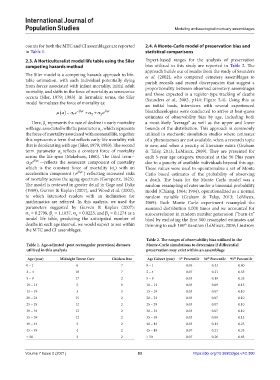
counts for both the MTC and CI assemblages are reported 2.4. A Monte-Carlo model of preservation bias and
in Table 1. statistical comparisons
2.3. A Horticulturalist model life table using the Siler Expert-based ranges for the analysis of preservation
competing hazards method bias utilized in this study are reported in Table 2. The
approach builds out of results from the study of Saunders
The Siler model is a competing hazards approach to life- et al. (2002), who compared cemetery assemblages to
table estimation, with each individual potentially dying parish records and record discrepancies that suggest a
from forces associated with infant mortality, initial adult proportionality between observed cemetery assemblages
mortality, and shifts in the force of mortality as senescence and those expected in a register-type tracking of deaths
occurs (Siler, 1979; 1983). In formulaic terms, the Siler (Saunders et al., 2002, p144: Figure 5.4). Using this as
model formulates the force of mortality as:
an initial basis, interviews with several experienced

a e 1 e bioarchaeologists were conducted to arrive at best-guess
3
2
1
2
estimates of observability bias by age, including both
Here, β represents the rate of decline in early mortality a most-likely “average” as well as the upper and lower
1
with age, associated with the parameter α , which represents bounds of the distribution. This approach is commonly
1
the force of mortality associated with neonatal life, together utilized in stochastic simulation studies where estimates
this represents a term that reflects early-life mortality risk of a phenomenon are not available, when a research topic
that is decelerating with age (Siler, 1979; 1983). The second is new, and when a paucity of literature exists (Graham
term parameter α reflects a constant force of mortality & Talay, 2013; LeMieux, 2009). They are presented for
2
across the life span (Makeham, 1860). The third term-- each 5-year age category, truncated at the 50 Plus years
e —reflects the senescent component of mortality due to a paucity of available individuals beyond this age.
3
2
which is the constant force of mortality (α ) with an These values were used to operationalize a set of Monte
2
acceleration component ( e ) reflecting increased risks Carlo based estimates of the probability of observing
3
of mortality across the aging spectrum (Gompertz, 1825). a death. The basis for the Monte Carlo model was a
The model is reviewed in greater detail in Gage and Dyke random resampling of rates under a binomial probability
(1989), Gurven & Kaplan (2007), and Wood et al. (2002), model (Chiang, 1964; 1984), operationalized as a normal
to which interested readers with an inclination for random variable (Graham & Talay, 2013; LeMieux,
mathematics are referred. In this analysis, we used the 2009). Each Monte Carlo experiment resampled the
parameters suggested by Gurven & Kaplan (2007): assumed distribution 1,000 times and we accounted for
α = 0.2798, β = 1.1037, α = 0.0223, and β = 0.1274 as a autocorrelation in random number generation (“burn-in”
1
2
3
1
model life table, predicting the anticipated number of bias) by excluding the first 500 resampled estimates and
deaths in each age interval, we would expect to see within thinning to each 100 iteration (LeMieux, 2009; Linstrom
th
the MTC and CI assemblages.
Table 2. The ranges of observability bias utilized in the
Table 1. Age‑adjusted (post rectangular proration) datasets Monte‑Carlo simulations to determine if differential
utilized in this analysis preservation may exist within an assemblage
Age (year) Midnight Terror Cave Chichen Itza Age Cohort (year) 5 Percentile 50 Percentile 95 Percentile
th
th
th
0 – 1 6 7 0 – 1 0.05 0.43 0.80
2 – 4 18 7 2 – 4 0.07 0.31 0.55
5 – 9 17 2 5 – 9 0.03 0.19 0.35
10 – 14 5 8 10 – 14 0.03 0.09 0.15
15 – 19 3 5 15 – 19 0.03 0.07 0.10
20 – 24 15 2 20 – 24 0.03 0.07 0.10
25 – 29 12 2 25 – 29 0.03 0.07 0.10
30 – 34 12 2 30 – 34 0.03 0.07 0.10
35 – 39 12 2 35 – 39 0.03 0.09 0.15
40 – 44 4 2 40 – 44 0.03 0.14 0.25
45 – 49 4 2 45 – 49 0.07 0.21 0.35
> 50 4 2 > 50 0.07 0.26 0.45

Volume 7 Issue 2 (2021) 83 https://doi.org/10.36922/ijps.v7i2.300