Page 84 - AJWEP-22-6

Heidarnejad, et al.

The influence of the gravitational acceleration gB 5 , C=F  w 1 , H d , w  (XI)

1

Q 2 d  B B w 2 
which represents the Froude number, is incorporated
through the dimensionless parameter H d . Given these 2.3. MLMs
B
conditions, Equation X is simplified to the following 2.3.1. SVM
41
Equation XI: Developed by Cortes and Vapnik, the SVMs are a
class of supervised learning methods used for
classification and regression tasks in machine learning.
A They are particularly well-suited for binary classification
problems, though extensions to multiclass classifications
exist. The core concept behind SVM is the construction
of hyperplanes in a high-dimensional space that can be
used to separate different classes of data points. Given
38
a training dataset {(X,y)} , where X ∈
N
n
i
i
i
i=1
represents the feature vectors and y ∈{-1,1} represents
i
the class labels, the objective of SVM is to find a
B
hyperplane that maximally separates the two classes. 42
To model a problem using SVM, the first step is to
clearly define the problem by determining whether it is a
classification, regression, or outlier detection task. Once
the task is identified, the next step involves collecting
and preprocessing the dataset to ensure that the data are
clean, normalized, and suitable for modeling. Based on
the nature and structure of the data, an appropriate kernel
function is then selected to transform the input space if
necessary. After selecting the kernel, the dataset is split
into training and testing sets, typically using an 80:20
ratio, to evaluate the model’s performance on unseen
data. The next step is to set the key hyperparameters
of the SVM model. These include the regularization
parameter C, which controls the trade-off between
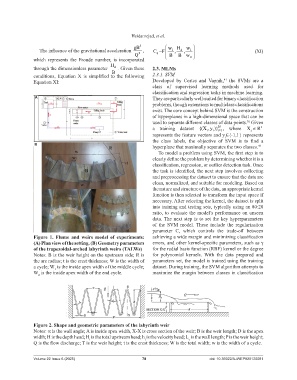
Figure 1. Flume and weirs model of experiments: achieving a wide margin and minimizing classification
(A) Plan view of the setting. (B) Geometry parameters errors, and other kernel-specific parameters, such as γ
of the trapezoidal-arched labyrinth weirs (TALWs) for the radial basis function (RBF) kernel or the degree
Notes: B is the weir height on the upstream side; R is for polynomial kernels. With the data prepared and
the arc radius; t is the crest thickness; W is the width of parameters set, the model is trained using the training
a cycle; W is the inside apex width of the middle cycle; dataset. During training, the SVM algorithm attempts to
1
W is the inside apex width of the end cycle. maximize the margin between classes in classification
2

Figure 2. Shape and geometric parameters of the labyrinth weir
Notes: α is the wall angle; A is inside apex width, X-X is cross section of the weir; B is the weir length; D is the apex
width; H is the depth head; H is the total upstream head; h is the velocity head; L is the wall length; P is the weir height;
t
t
c
Q is the flow discharge; T is the weir height; t is the crest thickness; W is the total width; w is the width of a cycle.

Volume 22 Issue 6 (2025) 78 doi: 10.36922/AJWEP025120081