Page 78 - IJAMD-2-2

International Journal of AI for
Materials and Design Prediction of AM defect based on DL

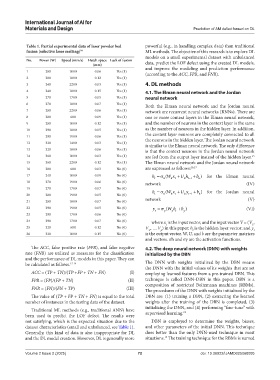
Table 1. Partial experimental data of laser powder bed powerful (e.g., in handling complex data) than traditional
fusion (selective laser melting) 10 ML methods. The objective of this research is to explore DL
models on a small experimental dataset with unbalanced
No. Power (W) Speed (mm/s) Hatch space Lack of fusion
(mm) data, predict the LOF defect using the created DL models,
1 200 1000 0.06 Yes (1) and improve the modeling and prediction performance
(according to the ACC, FPR, and FNR).
2 200 1800 0.12 Yes (1)
3 240 2200 0.03 Yes (1) 4. DL methods
4 240 1800 0.15 Yes (1) 4.1. The Elman neural network and the Jordan
5 270 1700 0.05 Yes (1) neural network
6 270 1800 0.07 Yes (1) Both the Elman neural network and the Jordan neural
7 280 2200 0.06 Yes (1) network are recurrent neural networks (RNNs). There are
8 280 600 0.09 Yes (1) one or more context layers in the Elman neural network,
9 280 1000 0.12 Yes (1) and the number of neurons in the context layer is the same
10 290 1800 0.05 Yes (1) as the number of neurons in the hidden layer. In addition,
11 290 1900 0.06 Yes (1) the context layer neurons are completely connected to all
12 320 1400 0.03 Yes (1) the neurons in the hidden layer. The Jordan neural network
is similar to the Elman neural network. The only difference
13 320 1800 0.06 Yes (1) is that the context neurons in the Jordan neural network
14 360 1000 0.03 Yes (1) are fed from the output layer instead of the hidden layer.
15
15 360 2200 0.12 Yes (1) The Elman neural network and the Jordan neural network
16 200 600 0.03 No (0) are expressed as follows: 16,17
17 240 1000 0.09 No (0) h =σ ( W x + U h + b ) for the Elman neural
ht −1
h
t
h
h
t
18 270 1900 0.06 No (0) network (IV)
19 270 1700 0.07 No (0) h =σ ( W x + U y + b ) for the Jordan neural
20 280 1900 0.05 No (0) t h h t h t −1 h
21 280 1800 0.07 No (0) network (V)
22 290 1900 0.05 No (0) y =σ ( W h + b ) (VI)
t
yt
y
y
23 290 1700 0.06 No (0)
24 290 1700 0.07 No (0) where x is the input vector, and the input vector V = (V ,
1
t
25 320 600 0.12 No (0) V ,…, V ) in this paper; h is the hidden layer vector; and y t
p
2
t
26 320 1000 0.15 No (0) is the output vector. W, U, and b are the parameter matrices
and vectors. σh and σy are the activation functions.
The ACC, false positive rate (FPR), and false negative 4.2. The deep neural network (DNN) with weights
rate (FNR) are utilized as measures for the classification initialized by the DBN
and the performance of DL models in this paper. They can
be calculated as follows. 12-14 The DNN with weights initialized by the DBN means
the DNN with the initial values of its weights that are set
ACC = (TP + TN)/(TP +FP + TN + FN) (I) employing learned features from a pre-trained DBN. This
FPR = (FP)/(FP + TN) (II) technique is called DNN-DBN in this paper. DBN is a
composition of restricted Boltzmann machines (RBMs).
FNR = (FN)/(FN + TP) (III) The procedures of the DNN with weights initialized by the
The value of (TP + FP + TN + FN) is equal to the total DBN are: (1) training a DBN, (2) extracting the learned
number of instances in the testing data of the dataset. weights after the training of the DBN is completed, (3)
Traditional ML methods (e.g., traditional ANN) have initializing the DNN, and (4) performing “fine-tune” with
18
been used to predict the LOF defect. The results were supervised learning.
not satisfying, which is the expected situation due to the DBN is employed to determine the weights, biases,
dataset characteristics (small and unbalanced, see Table 1). and other parameters of the initial DNN. This technique
Generally, this kind of data is also inappropriate for DL does better than the only DNN-used technique in most
and the DL model creation. However, DL is generally more situations. The training technique for the RBMs is named
19

Volume 2 Issue 2 (2025) 72 doi: 10.36922/IJAMD025060005