Page 102 - IJOCTA-15-1

´
R. Temoltzi-Avila, J. Temoltzi-Avila / IJOCTA, Vol.15, No.1, pp.92-102 (2025)
From (9) it follows that if we choose the external that is, we obtain the upper bound for y j ∈ Y δ j :
perturbations v ± , then the corre-
j ≡ ±δ j in V δ j δ j
sponding solutions of (8) are described by sup |y j (t)| ≤ 2 , (11)
t∈[0,T] κ 1 β j
t
Z
±
y (t) = ±δ j φ j (η)dη Furthermore, it can be verified that
j
0
˙ y j (t) = v j (t) − (2a j + µ α )y j (t)
δ j 2 1/2

= ± 1 − 1 − e j ψ j (t) Z
κ 1 β 2 t
j −µ α(t−η)
+ b j e y j (η)dη, (12)
where ψ j (t) = e −(µ α+a j )t cosh(c j t − arctanh(e j )) 0
and which allows us to conclude from (11) that

µ α a j − b j κ 2
e j = sup | ˙y j (t)| ≤ 2δ j 1 + . (13)
µ α c j t∈[0,T] κ 1
2

= sign (κ 1 − κ 2 )β − µ α · An application of the worst external perturba-
j
! −1/2 ±
4κ 1 κ 2 β 2 tions v j and the inequalities (11) and (13) is as
· 1 + j . follows. If we consider the reachability tube of (8)
2
((κ 1 − κ 2 )β − µ α ) 2
j α
Q = (t, y j (t)) : t ∈ [0, T] and y j ∈ Y δ j ,
We observe that e j ∈ (−1, 1). δ j
then its boundary is represented by the graphs of
+
y − and y , according to the inequalities given in
j
j
If we choose any other external perturbation v j ∈ (10). We observe that Q α is a simply connected
on the right hand-side of (8), and if y j is δ j
V δ j
set, symmetric with respect to the axis y j = 0
the corresponding solution associated with this α
+
−
choice, from the inequality v (t) ≤ v j (t) ≤ v (t) and bounded. In fact, the symmetry of Q δ j is
j j + −
valid for all t ∈ [0, T] and the definition (9), we obtained from the identity y (t) = −y (t) valid
j
j
obtain for all t ∈ [0, T]. Furthermore, to verify that Q α
δ j
−
+
y (t) ≤ y j (t) ≤ y (t), t ∈ [0, T]. (10) is simply connected, it suffices to note that if we
j j − +
choose τ ∈ [0, T] and ν ∈ [y (τ), y (τ)], then the
j
j
As a consequence of this geometric property, v − equality ˆy j (τ) = ν holds, where ˆy j ∈ Y δ j is the so-
j
and v + are called worst external perturbations. lution obtained by substituting the external per-
j
−
turbation ˆv j = θv + (1 − θ)v + into (8), where
j j
α
θ ∈ [0, 1], that is, it follows that (τ, ν) ∈ Q . Fi-
δ j
nally, we can observe from inequalities (11) and
(13) that
" #
Q α ⊂ [0, T] × − δ j , δ j ,
δ j 2 2
κ 1 β κ 1 β
j j
which shows that Q α is a bounded set.
δ j
The reachability tube Q α and the inequalities
δ j
(11) and (13) can be used to establish a robust
. We define the
stability criterion on the set Y δ j
:
following norm for y j ∈ Y δ j
∥y j ∥ = max {∥y j ∥ ∞ , ∥ ˙y j ∥ ∞ } ,
Y δ j
where ∥h j ∥ ∞ = sup t∈[0,T] |h j (t)|. According to
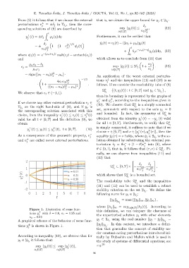
Figure 1. Illustration of some func-
± this definition, we can compare the closeness of
tions y with δ = 0.6, κ 1 = 0.35 and
j the unperturbed solution ¯y j with other elements
κ 2 = 0.15
=
A graphical scheme of the behavior of some func- using the real number ∥y j − ¯y j ∥ Y δ j
y j ∈ Y δ j
tions y ± is shown in Figure 1. ∥y j ∥ Y δ j . In this context, we introduce a defini-
j
tion that generalize the concept of stability un-
der constant-acting perturbations introduced ini-
According to inequality (10), we observe that for tially by Duboshin and Malkin which is used in
it follows that:
y j ∈ Y δ j the study of systems of differential equations; see
+
sup |y j (t)| ≤ sup |y (t)|, e.g. 26
j
t∈[0,T] t∈[0,T]
96