Page 66 - IJOCTA-15-1

O. Ayana, D. F. Kanbak, M. Kaya Keles / IJOCTA, Vol.15, No.1, pp.50-70 (2025)

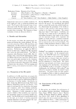
Table 2. The evaluation criteria’s formulas

Evaluation Criteria Formula of the Criteria
Accuracy (True Positive + True Negative) / (Positive + Negative)
Precision True Positive / (True Positive + False Positive)
Recall True Positive / Positive
F-score (2 * True Positive) / ((2 * True Positive) + False Positive + False Negative)

transactions’ users need to predict positively. F- For the BiLSTM model, we used the embedding
score comes into play in balancing precision and layer for the inputs. The embedding layer allows
recall. The F-score is the harmonic mean of pre- users to convert the words into a fixed-length vec-
cision and recall. For this reason, we make a per- tor, which learns the proximity of the words ac-
formance measurement by taking the F-score into cording to their position in the sentence and ac-
account when evaluating. The formulas of these cording to the degree of proximity. The embed-
evaluation criteria are shown in Table 2. ding layer takes 3 basic inputs: vocabulary size
(the first top-k unique words in the dataset), the
embedding dimension (the length of the vector),
4. Results and discussion and the maximum length which represents the
number of words used for a sentence/comment.
In this section, we define the experimental sce- The problem is that each sentence may not con-
narios and discuss the results obtained. We con- tain as many words as the maximum length. The
duct tests using four different ML algorithms, and example of this situation is shown in Table 3 (all
additionally, one DL model is proposed and pre- comments in the dataset may be with different
sented for comparative analysis with the ML al- lengths).
gorithms. Furthermore, we apply the BSO for
SA for the first time, utilizing the ML algorithm 87
Padding was employed to standardize each sen-
that yields the best performance. The BSO is
tence to a fixed length. In the proposed archi-
compared with Harmony Search (HS), Bat Al- tecture, two BiLSTM layers were implemented,
gorithm (BA), Atom Search Optimization (ASO)
with the unit kernel set as a parameter. Follow-
and Whale Optimization algorithm (WOA) which
ing these layers, a dropout layer was utilized to
have been previously presented in the literature
mitigate the risk of overfitting. The classification
and applied in the context of text mining. For all
process culminated in dense layers. The Adam
experiments conducted in this section, the dataset
optimizer was selected, and binary cross-entropy
is divided into two subsets: 70% for training and
was employed as the loss function. The structure
30% for testing, with scenarios executed on these
of the BiLSTM model is illustrated in Figure 2.
datasets. 88
Additionally, the GridSearch (GS) method was
utilized to accurately identify the model’s input
4.1. Parameters of the DL model parameters. The search space for each parame-
ter is detailed in Table 4, with the optimal values
determined by GS discussed in Section 4.2.3.
In addition to the ML algorithms, we propose the
use of one DL model that has garnered significant
attention recently and has demonstrated effective
performance in similar studies. Specifically, we
have chosen the Bidirectional Long Short-Term
4.2. Experiments of ML and DL
Memory (BiLSTM) model for this research. This
algorithms
choice is motivated by the observation that many
user comments, while often starting positively,
may conclude with a negative sentiment (or vice In this section, we evaluate the performance of
versa). Examples of such comments are illus- four machine learning algorithms: Multinomial
trated in Table 3. This variability can complicate Na¨ıve Bayes (MNB), Support Vector Machine
the algorithms’ ability to accurately classify com- (SVM), K-Nearest Neighbors (KNN), and Ran-
ments. The BiLSTM model is particularly suited dom Forest (RF). Each of these algorithms is
for this task, as it excels in learning sequential tested using the various preprocessing combina-
patterns inherent in text and possesses the capa- tions outlined in Table 1. Each combination C j
bility for bidirectional learning. 83–86 is represented by a code where 1 ≤ j ≤ 16, and
60