Page 153 - IJOCTA-15-2

A. Yoku¸s, H. Durur, M.H. Ekici / IJOCTA, Vol.15, No.2, pp.343-353 (2025)
2
Case 5: If property or behavior of the |u| wave function. In
particular, in fields such as wave theory or quan-
tum mechanics, the density of the wave function
√
48
2
− 18042 + 186i 31 k ln [a] 2 + represents the square of the amplitude.
v
1039417600m
u
u −
u
k 2
u
√
2
t 4 4
+ 18042 + 186i 31 k ln [a]
α 0 = ,
32240
21 2 √ 2
2
2
α 1 = 17k ln [a] + i 31k ln [a] ,
13
21 √
2
2
2
α 2 = − i −79ik ln [a] + 7 31k ln [a] 2 ,
13
84 2 2 √ 2 2
α 3 = 31k ln [a] + 3i 31k ln [a] ,
13
42 2 √ 2
2
2
α 4 = − i −31ik ln [a] + 3 31k ln [a] ,
13
v
u 1039417600m
−
u
16120v 2 − u k 2
u
k 2 t √ 2
4
+ 18042 + 186i 31 k ln [a] 4
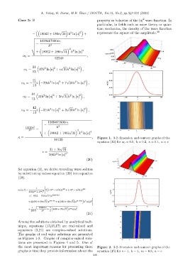
κ = , Figure 1. 3-2 dimension and contour graphs of the
16120
equation (13) for α 0 = 0.5, k = 0.2, κ = 0.1, a = e
√
31 + 3i 31
ϵ = 2 ,
2
260k ln [a]
(20)
for equation (1), we derive traveling wave soliton
by substituting values equation (20) into equation
(10).

"
1 √ √
u 5 (x, t) = 3 (−97 − i 31)a 4tv + (−97 − i 31)a 4kx
kx 4
tv
520(a + a )
√
+ (−8422 − 1126i 31)a 2(tv+kx)
#
√ √
2
+ 4(1093 + 69i 31)a 3tv+kx + 4(1093 + 69i 31)a tv+3kx k ln [a] 2
r
1 67600m 9 √
4
4
+ − + 4689 + 97i 31 k ln [a] .
260 k 2 2
(21)
Among the solutions obtained by analytical tech-
nique, equations (13,15,17) are real-valued and
equations (3,21) are complex-valued solutions.
The graphs of real value solutions are presented
as Figures 1-3. Graphs of complex-valued solu-
tions are presented in Figures 4 and 5. One of
the most important reasons for presenting these Figure 2. 3-2 dimension and contour graphs of the
graphs is that they provide information about the equation (15) for v= 1, k = 1, m = 0.8, a = e
348