Page 54 - IJOCTA-15-2

Multiple item economic lot sizing problem with inventory dependent demand
j J max
and is assumed to have a slope of a . To be it
it X j j
precise, this is how functions g it (), i = 1, . . . , N, U it = α u , i=1,...,N t=1,...,T, (11)
it it
t = 1, . . . , T, are defined: j=0
j
j
α ≤ v + v j+1 , i=1,...,N t=1,...,T j=1,...,J max −1
it it it it
(12)
g it (U) =
J max
it
0 X
d , U=u =0, v = 1, i=1,...,N t=1,...,T, (13)
0
j
it
it
j−1 j j−1 it
d it + a (U − u it ), u j−1 ≤U≤u , j=1,...,J it . j=1
j
max
it
it
it
max
J it
X
j
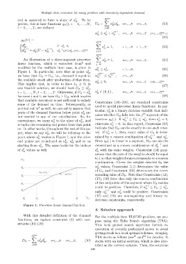
An illustration of a three-segment piecewise α = 1, i=1,...,N t=1,...,T, (14)
it
linear function, which is extracted from 4 and j=0
modified for the multiple item case, is given in α ≤ v , i=1,...,N, (15)
1
0
b
Figure 1. In particular, note that at point u , it max it max
it
we have that D it = U it , i.e., demand is equal to α J it it ≤ v J it , i=1,...,N (16)
it
the available stock after production of that item. j
α ≥ 0, i=1,...,N t=1,...,T j=0,...,J max
This implies that, in order to have I it ≥ 0, in it it (17)
b
any feasible solution, we should have U it ≥ u , j
it
i = 1, . . . , N, t = 1, . . . , T. Otherwise, if U it < u b v ∈ {0, 1} , i=1,...,N t=1,...,T j=1,...,J max
it it it
for some i and t, we have D it > U it , which implies (18)
that available inventory is not sufficient to satisfy
Constraints (10)–(18), are standard constraints
some of the demand on time. Subsequently, as used to model piecewise linear functions. In par-
4
pointed out in as well, we can safely assume that ticular, v is a binary decision variable that indi-
j
b
parts of the demand function below point u are it
it cates whether U it falls into the j th segment of the
not needed in any of our calculations. So, for j-1 j j
0
b
convenience, we carry u to the place of u , and function g it (.). If u it ≤ U it ≤ u , then v = 1;
it
it
it
it
j
re-index the remaining end points from that point otherwise v = 0. In that regard, Constraint (13)
it
on. In other words, throughout the rest of this pa- indicate that U it can be exactly in one such inter-
j
0
per, when we say u , we will be referring to the val. If v = 1, then, exact value of U it is deter-
it
it
j
b
point where u resides in Figure 1, and the other mined by a convex combination of u j−1 and u .
it it it
1
end points are re-indexed as u , u 2 and so on Since g it (.) is linear in a segment, D it can also be
it it
b
starting from u . The same holds for the indices determined as a convex combination of d j−1 and
it it
j j
of d values as well. d with the same weights. Constraint (14) guar-
it
it
antees that the sum of the weights should be equal
to 1 so that weighted sum corresponds to a convex
combination. Given the weights denoted by the
j
α values, Constraint (11) determines the value
it
of U it and Constraint (10) determines the corre-
sponding value of D it . Note that Constraints (12),
(15), (16) force that only the convex combination
of two endpoints of the segment where U it resides
j-1 j
could be positive. Therefore, if u it ≤ U it ≤ u ,
it
j−1 j
only α it and α could be positive. Constraints
it
(17) and (18) are nonnegativity and binary re-
striction constraints, respectively.
Figure 1. Piecewise linear demand function
4. Solution approach
With this detailed definition of the demand
For the multiple item ELSIDD problem, we pro-
functions, we replace constraint (4) with con-
pose using the Tabu Search algorithm (TSA).
straints (10)-(18):
This local guided search algorithm forbids re-
execution of recently performed moves to avoid
getting stuck in a local optimal solution. Roughly,
J max 81 82
it TSA works as follows (see and for details). It
X j j
D it = α d , i=1,...,N t=1,...,T, (10)
it it starts with an initial solution, which is also iden-
j=0 tified as the current solution. Then, the solutions
249