Page 57 - IJOCTA-15-2

¨
D. Balpınarlı, M. Onal / IJOCTA, Vol.15, No.2, pp.245-263 (2025)
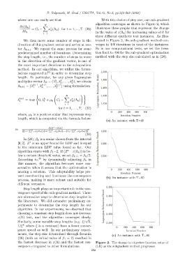
where one can easily see that With this choice of step size, our sub-gradient

N algorithm converges as shown in Figure 2, which
∂z(Λ k ) X
∗
= C t − x (Λ k ) for t = 1, ..., T. (26) illustrates three graphs that represent the change
it
∂λ t in the value of z(Λ k ) for increasing values of k for
i=1
three different synthetic test instances. As illus-
We then move some number of steps in the trated in Figure 2, the sub-gradient method con-
direction of this gradient vector and arrive at vec- verges in 400 iterations in most of the instances.
tor Λ k+1 . We repeat the same process for some So in our computational tests, we set the itera-
predetermined number of iterations. Determining tion limit to 400 for the sub-gradient optimization
the step length, i.e., the number of steps to move method with the step size calculated as in (28).
in the direction of the gradient vector, is one of
the most important decisions in the sub-gradient
method. In our algorithm, we utilize the formu-
lations suggested in 83 in order to determine step
length. In particular, for any given Lagrangian
k
k
k
multiplier vector Λ k = (λ , λ , . . . , λ ), we obtain
T
1
2
Λ k+1 = (λ k+1 , λ k+1 , . . . , λ k+1 ) using formulation
1 2 T
N
( !)
X
∗
λ k+1 k C t − x (Λ k )
t
t = max 0, λ + µ k it
i=1
for t = 1, . . . , T, (27)
where, µ k is a positive scalar that represents step
length, which is computed via the formula below:
(a) An instance with T=40
∗
β k (Z −z(Λ k ))
µ k = P N P N P N 2 .
∗
∗
∥(C 1 − i=1 x (Λ k )),(C 2 − i=1 x (Λ k )),...,(C T − i=1 x ∗ iT (Λ k ))∥
i1
i2
(28)
In (28), β k is a scalar chosen from the interval
∗
[0, 2]. Z is an upper bound for LDP and is equal
to the minimum LDP value found so far. Our
∗
algorithm starts with β 1 =2. If (Z −z(Λ k )) is be-
low a certain threshold value, we set β k+1 = β k /2.
According to, 46 by dynamically adjusting β k in
this manner, the algorithm becomes more con-
servative when it senses that the optimization is
nearing a solution. This adaptability helps pre-
vent overshooting and fine-tunes the convergence
(b) An instance with T=60
process, making it more robust and suitable for
different scenarios.
Step length plays an important role in the con-
vergence speed of the sub-gradient method. There
are alternative ways to determine step lengths in
the literature. We did extensive preliminary ex-
periments to determine the step length for our
algorithm. In our experiments, we observed that
choosing a constant step length does not decrease
z(Λ) fast, and the algorithm converges slowly.
√
Similarly, some variable step lengths (e.g. ξ/ k,
k
1/ξ where ξ is a constant) have a lower conver-
gence speed as well. In our preliminary experi-
ments, the step size determined through formula
(c) An instance with T=80
(28) (with an initial value of β 1 = 2) resulted in
the fastest decrease in z(Λ) and the fastest con- Figure 2. The change in objective function value of
vergence compared to other formulations. (LR) as the subgradient method progresses
252