Page 60 - IJOCTA-15-2

Multiple item economic lot sizing problem with inventory dependent demand
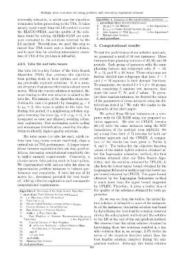
inherently infeasible, in which case the algorithm Algorithm 4. Summary of the overall solution procedure.
terminates before proceeding to the TSA. It takes 1: procedure Main Algorithm(Dataset)
2: (y 1 ,y 2 ) ← LR Method ▷ See Algorithm 1
usually much longer than the LR method to solve 3: y initial ← Create Hybrid Solution (y 1 , y 2 )
the ELSIDD-FEAS, and the profits of the solu- 4: Best Solution ← TSA (y initial ) ▷ See Algorithm 3
tions found by solving ELSIDD-FEAS are quite 5: Return Best Solution
6: end procedure
poor compared to the solutions returned by the
LR method. Nevertheless, we need this step to
5. Computational results
ensure that TSA starts with a feasible solution,
and to save time by avoiding unnecessary execu- To test the performance of our solution approach,
tion of TSA if the problem is infeasible. we generated a total of 90 test instances. These
instances have planning horizons of 40, 60, and 80
4.2.3. Tabu list and tabu tenure periods. Each group of instances with the same
planning horizon has subgroups with N = 10,
The tabu list is a key feature of the Tabu Search
N = 15, and N = 20 items. These subgroups are
Algorithm (TSA) that prevents the algorithm
further divided into subgroups that have J = 5
from getting stuck in local optima and revisit-
and J = 10 segments in their demand functions.
ing previously explored solutions. It is a mem-
To summarize, we created 3 × 3 × 2 = 18 groups,
ory structure that stores information about recent
each containing 5 random test instances, that
moves. When the current solution is updated, the
share the same T, N, and J values. To gener-
move leading to the new solution is added to the
ate these random instances, we derived the values
tabu list. For instance, if the algorithm stops pro-
of the parameters of these instances using the dis-
duction for item i in period t by changing y it = 1 4
tributions stated in. We refer the reader to the
to y it = 0, this move is added to the tabu list.
Appendix of the cited paper.
During this period, if a neighboring solution sug-
We solved these 90 test instances on a com-
gests reversing the move (y it = 0 → y it = 1), it is
puter with 64 GB RAM using our proposed so-
recognized as tabu and skipped, avoiding redun-
lution approach. We also let CPLEX (version
dant exploration. This mechanism avoids cycling
20.1.0) solve the same instances using the MIP
and encourages diversification, enabling the algo-
formulation of the multiple item ELSIDD. We
rithm to identify higher-quality solutions.
set a total time limit of 15 minutes for both our
The tabu tenure (or tabu list size), which de-
solution approach and the CPLEX. A compar-
fines how long moves remain restricted, plays a
ison of the results has been given in Tables 3,
critical role in TSA performance. A longer tenure
4, and 5. The tables list the objective function
allows broader exploration but can skip good so- values of the initial hybrid solution obtained af-
lutions, increasing computational complexity due ter the Lagrangian relaxation method, the final
to higher memory requirements. Conversely, a solution obtained after our Tabu Search Algo-
shorter tenure risks getting stuck in local optima. rithm, and the solution obtained by CPLEX. It
We experimented with various tabu list sizes on
also lists the lowest upper bound obtained by the
representative problem instances to balance per-
Lagrangian Relaxation method and the lowest up-
formance and complexity. A tabu list size of 20
per bound obtained by CPLEX. The upper bound
moves (i.e., iterations) provided the best trade-
obtained by the Lagrangian Relaxation method
off, offering effective exploration and manageable
is much lower than the upper bound suggested
computational requirements.
by CPLEX. Therefore, it gives a better idea of
Algorithm 3. Summary of the Tabu Search Algorithm. the quality of the solutions obtained for both ap-
1: procedure Tabu Search Algorithm(y initial ) proaches.
2: t ← End time of the LR method As we can see from the tables, the initial hy-
3: Tabu List ← {}
4: Obtain Initial Solution corresponding to y initial brid solution is infeasible in none of the instances.
5: Current Solution ← Initial Solution In all the instances, this initial solution was found
6: Best Solution ← Current Solution by hybridizing the best feasible solution observed
7: while t ≤ Time Limit do
8: Best Neighbor ← Search Neighborhood(y current, during the sub-gradient method and the solution
Tabu List) ▷ See Algorithm 2 to the LR at the end of the sub-gradient method.
9: Current Solution ← Best Neighbor We observed that this initial solution obtained by
10: if z(Current Solution) > z(Best Solution) then
11: Best Solution ← Current Solution hybridizing these two solutions resulted in a fea-
12: end if sible solution that is, on average, 2.5% better (in
13: t ← get time terms of the objective function value) than the
14: end while best feasible solution observed during the sub-
15: Return Best Solution
16: end procedure gradient method. Although this initial solution
255