Page 61 - IJOCTA-15-2

¨
D. Balpınarlı, M. Onal / IJOCTA, Vol.15, No.2, pp.245-263 (2025)
is, on average, 14% worse than the solution found We can see from Table 6 that both CPLEX
by CPLEX in terms of objective function value, in and our approach are affected by problem size,
11 out of 90 instances, it is better than the final which can be defined by three key factors: T,
solution of the CPLEX. Noting that it takes at N and J. Although the gap results of both ap-
most 15 seconds to execute, these results indicate proaches increase by problem size, the dominance
the efficacy of the Lagrangian relaxation method of our approach on CPLEX is maintained. In or-
in feeding good initial solutions to the TSA. We der to determine the effects of these factors on the
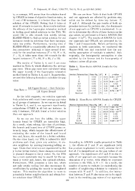
would like to also remark that merely solving gap values, we performed a 3-factor ANOVA (See
84
ELSIDD-FEAS to find an initial solution for our chapter 14 in ). The results of ANOVA for both
instances result in solutions that have incompa- our approach and CPLEX are presented in Ta-
rably low profits. Furthermore, running time of bles 1 and 2 respectively. Before performing the
ELSIDD-FEAS is considerably affected by prob- analysis in both approaches, we conducted the
lem parameters: although it takes around 4 sec- Shapiro-Wilk test and concluded that the nor-
onds for the smallest instances (T = 40, N = 10, mality assumption of residuals is satisfied. Sub-
J = 5), it takes more than 160 seconds for the sequently, the homogeneity assumption is also
largest instances ( T = 80, N = 20, J = 10). satisfied by the Levene test for homogeneity of
variance across all groups.
The results of Tables 3, 4, and 5 are sum-
marized in Table 6, which illustrates the average Table 1. Three-Factor ANOVA Results for Our
gap rates. These gap rates were calculated using Approach
the upper bounds of the Lagrangian relaxation
method listed in Tables 3, 4, and 5. In particular, Factor/Interaction Sum Sq. df F p-value
we used the following formula to calculate the gap T 0.042 2 43.01 5.13 × 10 −13
J 0.001 1 2.17 0.145
rates: N 0.091 2 93.57 9.48 × 10 −21
T:J 0.001 2 1.12 0.333
T:N 0.018 4 9.38 3.69 × 10 −6
LR Upper Bound − Best Solution J:N 0.001 2 1.15 0.323
Gap Rate = −3
LR Upper Bound T:J:N 0.007 4 3.68 8.74 × 10
Residual 0.035 72 −− −−
As the table suggests, our solution approach
finds solutions with much lower average gap rates Table 2. Three-Factor ANOVA Results for CPLEX
in all groups of instances. As we can see in detail
in Tables 3, 4, and 5, our approach significantly Factor/Interaction Sum Sq. df F p-value
T 0.106 2 41.12 1.23 × 10 −12
outperforms CPLEX in all but one instance: in −4
J 0.018 1 14.15 3.41 × 10
only 1 instance, CPLEX found a better solution N 0.435 2 168.69 6.72 × 10 −28
than our approach. T:J 0.002 2 0.92 0.401
T:N 0.008 4 1.65 0.172
As we can see from the tables, the upper J:N 0.007 2 3.01 0.0556 −3
bounds found by CPLEX are incredibly high. T:J:N 0.022 4 4.35 3.29 × 10
Residual 0.092 72 −− −−
As a result, when solving this class of problems,
the branch and bound tree of CPLEX grows ex-
tremely large, which impairs the effectiveness of
evaluating the nodes of the branch and bound
tree and, hence, the search for a better solution.
On the other hand, our TSA is tailored for ELS
problems such that, given any solution, it cre- According to ANOVA results presented in Table
ates neighbors by moving/removing/adding se- 1, the effects of T and N are significant (with
tups. Given that solutions are represented by the low p-values emphasized in bold), whereas the ef-
y vector (setup vector), these changes correspond fect of J is insignificant on the gap values of our
to planned changes in the y vector. So, the TSA approach. The significance of T and N on the re-
has a more systematic way to search for the op- sults of our approach are reasonable because the
timal y vector and, hence, the optimal solution. dimension of y vector, with which we represent
Furthermore, TSA possesses a tabu list, which solutions in the TSA, is N × T. As a result, the
not only avoids cycling but also encourages di- number of moves to evaluate (or equivalently, the
versification by guiding the search to unexplored number of neighboring solutions to evaluate) in-
regions. This enables the algorithm to move to creases with N and T. In addition, the interac-
potentially better neighborhoods and obtain bet- tion between T and N also turns out to be signif-
ter solutions than CPLEX. icant in the resulting gap values of our approach.
256