Page 62 - IJOCTA-15-2

Multiple item economic lot sizing problem with inventory dependent demand
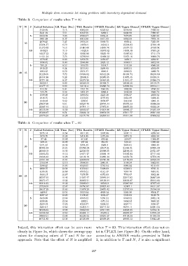
Table 3. Comparison of results when T = 40

T N J Initial Solution LR Time (Sec) TSA Results CPLEX Results LR Upper Bound CPLEX Upper Bound
5139.82 7.15 6362.08 6225.62 6442.98 7496.50
5331.32 7.51 6337.56 6283.5 6494.98 7956.87
5 6043.58 7.86 6980.07 6862.21 7076.65 8246.84
5461.68 8.37 6816.88 6611.43 6955.08 7879.19
4978.45 7.47 5956.36 5890.75 6050.4 7255.09
10
15294.57 6.79 14654.9 14142.3 15204.03 17396.48
15172.82 7.15 15410.96 14895.76 15577.32 17540.04
10 15492.9 7.19 14323.8 13973.52 14895.48 17699.24
16027.23 7.30 15930.88 15530.49 15987.62 17121.79
14151.24 7.73 15789.94 15468.53 15973.16 16888.76
1578.65 8.89 2356.79 2258.67 2456.3 4223.81
1696.42 8.40 2940.48 2828.12 3068.01 4412.58
5 785.25 8.53 1050.75 1014.7 1101.58 4546.59
1812.35 9.24 2533.81 2499.92 2693.51 4502.69
1964.53 8.70 3071.77 2940.8 3208.55 4488.78
40 15
23128.05 7.72 33309.92 31512.28 36469.74 38190.80
26444.86 9.28 29306.8 26985.05 31075.45 34330.91
10 25771.95 8.27 29279.28 28464.85 31542.47 34586.79
23559.4 8.89 26305.59 26498.71 28500.25 29149.74
23277.15 8.09 22139.4 20226.74 23066.84 26614.11
813.59 9.41 1721.79 1546.95 1882.06 3796.23
735.78 9.56 1451.27 1266.4 1535.58 3566.73
5 1599.66 10.25 2880.82 2425.28 3092.27 4609.04
1916.75 9.16 3153.56 2797.03 3451.09 5492.35
1543.48 9.62 2266.6 2030.87 2412.56 4949.15
20
27837.89 9.51 36527.75 29784.44 39973.33 40980.03
25967.44 10.13 34714.11 27972.91 38075.58 40929.94
10 20535.98 10.59 26802.87 24004.86 29086.27 34265.89
25288.67 8.74 32603.13 29874.59 37011.77 39501.68
23576.23 10.25 32170.79 26205.53 35911.98 37484.82
Table 4. Comparison of results when T = 60

T N J Initial Solution LR Time (Sec) TSA Results CPLEX Results LR Upper Bound CPLEX Upper Bound
2075.14 10.54 3011.95 2907.06 3097.11 4269.93
1878.70 11.93 2414.45 2372.06 2478.12 4853.94
5 87.44 10.68 213.26 209.42 220.97 1392.29
208.14 11.66 497.32 481.05 520.13 1080.22
2171.43 11.49 2394.49 2388.3 2600.81 3999.30
10
20982.59 10.21 20,798.24 19517.21 21466.91 23825.20
20060.19 11.40 22036.58 20096.05 22500.35 24721.87
10 22993.53 11.13 24071.27 22088.19 24365.03 27171.66
22646.42 10.28 24102.16 23260.34 24359.76 27756.96
23561.94 10.81 22608.63 21740.46 23150.69 26928.03
2193.54 12.13 3088.99 2843.91 3188.34 5662.60
3566.45 10.90 6049.05 5785.64 6680.24 8110.60
5 2899.75 12.04 6156.93 5408.69 6508.01 9745.11
4108.55 11.88 6939.21 6141.47 7267.78 9481.01
5534.17 11.87 7178.78 6372.63 7705.07 9342.36
60 15
30597.92 11.46 31587.47 29949.04 33917.82 36867.09
28372.47 12.33 30862.21 29138.04 33629.87 35012.83
10 29214.63 11.38 32828.61 28536.9 35847.02 37677.43
27720.38 12.47 30750.87 28827.43 32967.1 34311.67
28637.28 11.60 31674.29 29470.42 33767.69 35184.99
4499.5 12.51 5023.04 4020.14 5241.56 9504.37
4387.13 12.20 5138.25 4692.27 5540.94 9158.78
5 5343.69 12.69 6065.52 5256.24 6568.52 10821.34
4408.65 12.55 4932.5 4471.54 5653.53 9650.22
5334.02 12.82 6232.57 5090.22 6587.71 9250.87
20
33616.4 12.50 42218.41 35717.22 46744.11 50981.53
30996.63 12.86 39655.99 32911.69 44026.65 52724.34
10 33098.54 12.60 43484.11 35259.4 48876.87 53579.29
34889.21 13.43 42226.32 35581.27 47198.56 51398.90
40731.85 12.36 45320.66 41039.49 49865.12 53043.48

Indeed, this interaction effect can be seen more when T = 80. This interaction effect does not ex-
clearly in Figure 3a, which shows the average gap ist in CPLEX (see Figure 3b). On the other hand,
values for changing values of T and N for our according to ANOVA results presented in Table
approach. Note that the effect of N is amplified 2, in addition to T and N, J is also a significant

257