Page 55 - IJOCTA-15-2

¨
D. Balpınarlı, M. Onal / IJOCTA, Vol.15, No.2, pp.245-263 (2025)
in the neighborhood of this current solution are that makes them a good fit for applying the La-
evaluated. The best solution in the current solu- grangian relaxation method. In such problems,
tion’s neighborhood is selected and becomes the capacity constraints usually tie a set of single item
new current solution. This process of evaluating (uncapacitated) ELS problems. Hence, if those
the neighborhood is repeated with the new cur- tying capacity constraints are dualized, the cor-
rent solution, and the process continues. Here, responding LR solves a set of independent single
the neighborhood of a solution is a set of solutions item ELS sub-problems. Most of the time, these
that can be obtained by making small changes in subproblems can be solved in polynomial time,
the current solution. Throughout this procedure, implying that the LR of multiple item ELS prob-
the best solution is stored and updated whenever lems can be solved easily.
a better solution is found. With the operations
In the multiple item ELSIDD problem, these
defined in this manner, the process might get eas-
tying constraints are Constraints (5), i.e., produc-
ily stuck in a local optimal solution. TSA avoids
such a detriment by creating a memory structure tion capacity constraints. It is easy to see that if
that forbids moves which lead back to local opti- these constraints are removed, the problem de-
mal solutions. When a predetermined criterion is composes into N independent single item unca-
4
met, or if it is not possible to improve the solution pacitated ELSIDD problems, for which propose
found in a predetermined number of iterations, a polynomial time dynamic programming algo-
the process is terminated, and the best solution rithm. In our Lagrangian relaxation method, we
4
is presented. utilize the algorithm of to solve the single item
sub-problems, hence the LR.
Initial solutions significantly influence the
performance of the TSA. Therefore, before start-
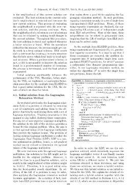
ing the TSA, we implement a Lagrangian Relax- Algorithm 1. Summary of Lagrangian relaxation method.
ation procedure for the multiple item ELSIDD to 1: procedure Lagrangian Relaxation Method
2: k ← 1
find a good initial solution for the TSA, the de- 3: Λ k ← 0 ▷ Initial Lagrange multiplier vector set to 0
tails of which we describe below. 4: β k ← 2 ▷ Initial β param. of the Subg. Opt. Meth.
5: y LagBest ← null ▷ Initially, y LagBest is set to null.
4.1. Initial solution from the Lagrangian 6: z Best ← −∞
Relaxation Method 7: while k ≤ max. iteration number do ▷ 400 iter.
∗
∗
8: Solve z(Λ k) and obtain x (Λ k), y (Λ k)
∗
As we stated previously, the Lagrangian relax- 9: if y (Λ k) is feasible then
∗
10: if z(y (Λ k)) > z Best then
ation (LR) of a problem is obtained by removing ∗
11: y LagBest ← y (Λ k)
a set of constraints and adding them to the ob-
12: end if
jective function by multiplying them with a set of 13: end if
∗
Lagrange multipliers. Treating constraints in this 14: procedure Subgradient Optimization(x (Λ k ))
manner is also called dualizing those constraints. 15: Determine step length µ k using (28)
16: Determine Λ k+1 using (27)
For any set of non-negative Lagrange multipliers, 17: Set β k+1 = β k /2 if (Z − Z(Λ k )) ≤ threshold
∗
the solution to the LR of the problem provides a 18: end procedure
bound for the original problem. Then, the aim is 19: Increment k
20: end while
to find optimal values of the Lagrange multipliers 21: if y LagBest not null then
that provide the tightest bound. The problem of 22: Return y LagBest , y (Λ 400 )
∗
∗
∗
finding optimal Lagrange multipliers is called the 23: Else Return y (Λ 100 ), y (Λ 400 )
24: end if
Lagrangian Dual Problem (LDP). LDP is a con-
25: end procedure
vex optimization problem, hence, a sub-gradient
method can be utilized to determine the optimal
values of the Lagrange multipliers. In order to solve the LDP, we use the sub-
We note that even with the optimal Lagrange gradient method, which iteratively improves the
multipliers, the solution to the LR might not be Lagrange multiplier vector Λ and finally reaches
feasible for the original problem. However, it the optimal vector Λ. At each iteration, LDP
could be close to a good feasible solution, and a solves LR for a different vector Λ. We pick two
search in the neighborhood of this solution might solutions obtained in these iterations, and using
be fruitful. Therefore, it is a good initial solu- these two solutions, we create a hybrid solution.
tion for local-guided search algorithms. In ad- We then use this hybrid solution as an initial so-
dition, if the LR of a problem is easy to solve, lution for the TSA. We explain the details of ob-
then applying the Lagrangian relaxation method taining such a hybrid solution together with the
becomes appropriate. As a matter of fact, mul- details of our LR method in Sections 4.1.1, 4.1.2
tiple item ELS problems have a special structure and 4.1.3, which we also summarize in Algorithm
250