Page 114 - IJOCTA-15-4

Zhang et al. / IJOCTA, Vol.15, No.4, pp.649-669 (2025)

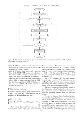
Figure 2. A flowchart illustrating the golden sine subtraction-average-based optimizer (GSABO)–back-
propagation (BP) neural network

• Step 4: MFE is used to extract features from bearing failures. The following are the parame-
reconstructed signals and construct feature sets ters: sampling frequency fs = 1200 Hz, number
representing different states. of sample points N = 6000, fault impact dura-
• Step 5: With the state feature set learned in tion T = 0.01 s, fault characteristic frequency f
Step 4, the GSABO–BP neural network classi- = 1/T = 100 Hz, natural frequency f n = 3000
fier can be guided during the classification pro- Hz, displacement constant A 0 = 5, and damping
cess. This structured approach enhances fault coefficient g = 0.1.
diagnosis accuracy by leveraging the strengths Figure 4 illustrates the simulated signal’s
of the GJO for parameter optimization, VMD time-domain waveform. The noise obscures the
for signal decomposition, MFE for feature ex- rolling bearing’s periodic impact characteristics,
traction, and GSABO–BP neural network for inevitably diminishing the accuracy of the subse-
feature classification. quent signal feature extraction process.
The most popular and user-friendly technique
4. Simulation analysis for diagnosing rolling bearing faults is the enve-
lope spectrum approach. Figure 5 presents the
To validate the effectiveness of the VMD method,
envelope spectrum obtained from the simulated
an early fault signal for rolling bearings was es-
signal.
tablished, as shown in Equation (13):
In order to diagnose the rolling bearing fault,
the simulated signal y(t) must be processed to re-
y(t) = x(t) + n(t)

 move interference components and enhance the
X p
2
x(t) = e −2πf ngt 0 · A 0 sin[2πf n (1 − g ) · t 0 ] accuracy of fault feature extraction. As illus-

i trated in Figure 5, background noise causes the
(13) spectral line at the fault characteristic frequency
where n(t) is Gaussian white noise, and x(t) in the envelope spectrum to be less prominent.
is the periodic impact signal produced by rolling With significant interference present, identifying
656