Page 89 - IJPS-10-2

International Journal of
Population Studies Employment-driving effect

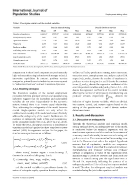
Table 1. Descriptive statistics of the studied variables
Variable Panel A: Manufacturing Panel B: Producer services
Mean SD Min Max Mean SD Min Max
Number of employees 11063.17 17095.57 119.00 168600.00 12334.02 29573.61 105.00 293592.00
Enterprise equity nature 0.68 0.47 0.00 1.00 0.70 0.46 0.00 1.00
Operation duration 21.26 5.91 7.00 40.00 20.85 6.84 3.00 39.00
Wage level 11.99 0.45 10.61 13.33 12.04 0.52 10.07 13.73
Employee welfare 0.75 0.44 0.00 1.00 0.73 0.45 0.00 1.00
Staff safety production training 0.58 0.49 0.00 1.00 0.63 0.48 0.00 1.00
R&D innovation 47742.11 104397.89 0.00 1496713.48 45286.18 159213.23 0.11 2187415.10
Log of enterprise assets 23.40 1.35 20.52 27.55 23.71 1.42 19.83 27.81
Unemployment rate 3.03 0.74 1.21 4.61 2.95 0.79 1.21 4.61
GDP per capita 105727.12 42890.03 19436.00 203489.00 121676.24 41270.41 16248.00 467749.00
Notes: R&D: Research and development; GDP: Gross domestic product; SD: Standard deviation.

companies in A-share listed companies are predominantly welfare, staff safety production training, R&D innovation,
high-tech manufacturing industries with stronger technical enterprise assets, unemployment rate, and per capita GDP,
innovation capabilities. In contrast, producer services respectively. produc denotes the number of employees in
i
companies, primarily service industries, are more exposed producer services in region i, α, and ∂ denote the constant
to “subservient business” and lack innovation dynamics. terms, β and ρ denote the regression coefficient of the
0
0
core independent variables, and β and ρ (for i=1,2,3,…,10)
i
2.3.2. Modeling strategies denote the regression coefficients of the control variables
i
The theoretical analysis of the mutual employment affecting the number of employees in manufacturing and
3
promotion between producer services and manufacturing producer services, respectively. area denotes the
industries suggests that the dependent and independent k1 k
variables do not exist independently in the economic inclusion of region dummy variables, which are divided
system; instead, there is an inverse causal relationship. into eastern, central, and western regions based on the
Thus, addressing the endogeneity of the model becomes setting of the questionnaire. ε and δ denote random
crucial. Single-equation models can only reflect the disturbance terms.
unidirectional causality of the model and cannot effectively
address the endogeneity of the model. Furthermore, the 3. Results and discussion
existence of endogeneity leads to bias and inconsistency 3.1. Discussion on endogeneity
in the estimation results (Pan et al., 2019; Yu et al., 2018).
To tackle this issue, this paper constructs a simultaneous Through the theoretical analysis and empirical model
equations model and applies the three-stage least squares setting outlined above, an endogeneity test of the model
method (3SLS) for regression analysis. In this paper, the is conducted before the empirical regression with the
simultaneous equations are set as follows: simultaneous equations model to confirm the existence of
a two-way causal relationship between manufacturing and
3 producer services. The common method for an endogenous
i
manuf 0 produc i Z area
i
i
k
k1 test is the Hausman test, where the original hypothesis
3 (XIV) assumes that all explanatory variables are exogenous.
produc manuf Z area
i i
i 0 i i k The results in Table 2 show that the relationship between

k1
manufacturing and producer services and producer
where manuf denotes region i manufacturing. Z i services is exogenous. p-values of the regressions from
i
denotes the control variable group, that is, manufacturing to producer services and from producer
Z = ( ownership time wage welfaretrain i i i i i services to manufacturing pass the significance tests at
i
innovassetjoobless perGDP ) (XV) 5% and 1%, respectively, indicating the presence of an

endogeneity problem if the ordinary least squares method
i
i
i
i
and the control variables in parentheses denote the is used. Therefore, the subsequent empirical analysis was
nature of enterprise equity, operation duration, employee conducted using the joint cubic equation model.
Volume 10 Issue 2 (2024) 83 https://doi.org/10.36922/ijps.0316