Page 95 - IJPS-10-4

International Journal of
Population Studies Mortality shapes population age structures

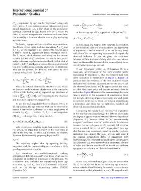
(P – population by age) can be “explained” using only P L
x
*
the L series. A close correspondence between reality and OADI P 65 ; OADI L 65 (IV)
x
model predictions (i.e., a high share of the population 15 64 15 64
correctly classified by age, based only on a recent life or the average age of the population, A (Equation V):
table) is, in our interpretation, consistent with our claim
that mortality is the most relevant force at play in shaping A xc A ; * xc * (V)
age structures. x x
To develop our approach, we introduce some notations. In both cases, the purpose is to compare the evolution
We denote vectors using bold font and define P = P and of the asterisked indicator (which follows our hypothesis
t
x,t
L = L , as the population and years of life lived at age x of Equation III and is assumed to be the driving force)
t
x,t
at time t (where L , signifies the period ending in year t). with that of the corresponding non-asterisked empirically
t
The L series, which depends exclusively on the current observed indicator. In practice, given the consistent
t
survival (or mortality) conditions, can also be interpreted behavior of these indicators (along with others not shown
as the stationary population associated with the life table of here), as discussed in Section 3.1, the focus will only be on
period t. Both P and L encompass a dimensional element one of them, the average age (A).
t
t
that is to be eliminated, focusing exclusively on structures.
This can be achieved by dividing both series by their If our hypothesis holds, i.e., if Equation III is a
corresponding totals (Equation I): reasonable approximation of the more complex reality
represented by Equation II, what we expect to find with
P L these indicators is exemplified in Figure 1. Figure 1A
c c xt, and c c * xt , (I) predicts that the evolution of the two indicators (same
*
x xt , t x t , x xt , indicator but calculated separately on the stationary and
t
x t,
L
P
where the asterisk denotes the stationary case, which the observed population) will be approximately the same,
we interpret as the standard of reference in the remainder i.e., that their time paths will remain relatively close to
of this article. Both c and c represent age structures at each other. Figure 1B conveys the same message, but now
*
t
t
time t x x * 1 , corresponding to the observed time is implicit in the succession of observations (from
c
c
and stationary population, respectively. left to right, denoting improved survival), and each point
is expected to lie not far from the bisector, representing
As per the weak ergodicity theorem (Lopez, 1961), in a theoretical case where the two indicators, standard and
all populations, the age structure that can be observed at observed, possess identical values.
instant t, denoted as c , depends on a very long history of Comparing the standard and the observed population
t
*
*
survival ( cc, t 1 ,), fertility (F , F ,…), and migration in this way has one disadvantage: it is difficult to evaluate
t-1
t
t
(M , M ,…) from periods ending in t, t-1,… the degree of approximation introduced by our hypothesis
t
t-1
(Equation III) because there is no conventionally
*
)
c =f( c FM cF,, t t ; t * -1 t-1 , M ;.… (II) accepted “confidence interval” within which the distance
t-1
t
t
between the two indicators should normally fall. Another
with recent years weighing more than remote ones. In minor drawback is the risk of “compensation”: two age
this article, we argue that mortality is the main force at distributions may occasionally result in similar synthetic
play in the long run. To prove our assertion, we simplify indicators (e.g., almost the same average age) even if
Equation II considerably, proposing Equation III:
the original distributions differ. To circumvent both
c ≈ c * t (III) shortcomings, we computed the index of the dissimilarity,
t
The equation implies that by ignoring fertility, ID (Equation VI), which provides the proportion of units
migration, and also past mortality; we can achieve a fairly of either distribution that should be moved to a different
good approximation of reality. age groups to make the two distributions identical.
Age structures are multidimensional, making 1 *
comparisons difficult, especially over time, which can be ID 2 c c x (VI)
x
x
considered an additional dimension of the problem. We
circumvent this difficulty by transforming both age In our case, without loss of generality, we assume that
*
*
structures, c and c , into one-dimensional indicators, the c series, derived from the stationary age structure,
t
t
t
such as the old-age dependency index (OADI) acts as a standard and that only the units in c can and must
t
*
(Equation IV): be relocated, so that, ultimately, c = c . ID ranges from 0,
t
t
Volume 10 Issue 4 (2024) 89 https://doi.org/10.36922/ijps.377