Page 59 - IJPS-11-1

International Journal of
Population Studies Macroeconomic factors and housing dynamics

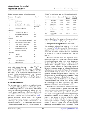
Table 1. Parameter values of the benchmark model Table 2. The equilibrium value set of the benchmark model
Parameter Description Value (%) Variables Description Benchmark Population Technology
Demographics decline ‑enhanced
J Maximum age 65 r* Interest rate 0.0649 0.0590 0.1144
Jr Retirement age 45 ph* House price 1.4145 1.4145 1.3769
πj Conditional survival possibilities Actuarial Life tr* Government 0.4189 0.4857 0.5424
Table (2021) transfer
n Population growth rate 0 w* Wage income 5.6430 5.7705 8.0006
Preferences b* Social security 2.5869 1.9385 3.6677
payment
Σ Coefficient of risk aversion 2
Bene Social security 2973.17 2802.77 4215.35
χ Share of non-durable goods 0.85 account
Β Discount factor 0.97
Production simulate the effects of an aging population through early
α Capital share in consumption sector 0.35 retirement, with Table 3 highlighting its impacts.
ϕ Non-land share in housing sector 0.9
ν Capital share in housing sector 0.3 3.1. Comparison among alternative economies
δ Capital depreciation rate 0.081 The equilibrium values of our price set {r*,p *,tr*,w*},
h
δh Housing depreciation rate 0.023 are presented in Table 2. Demographic change causes the
g Technology growth rate 0 aggregate social security stock to decrease at the same rate
Government as the total population. With this balanced growth path,
we detrend the data and take the average over a long time
pl Land price 1
interval.
τ Payroll tax rate 12.4
The second column shows that population decline
Market has no effect on house prices in this deterministic model.
λ Down payment ratio 20 A possible explanation is that construction firms reduce
τh Transaction cost 6 the pace of new housing projects to align with falling
demand. Since demographic changes are predictable, the
of the Cobb–Douglas function. Y 1 to aggregate demand is known to construction companies.

c
c
c
c
N
Z K
t
t
t
t
match the U.S. NIPA data. The average capital-income Moreover, the model assumes an unlimited land supply,
so land prices remain unaffected by population changes.
share, α, is set equal to 0.35 between 1954 and 2018. The The interest rate drops by around 9% due to decreased
land share (1−ϕ) in the construction industry is set to 10% aggregate demand, leading to reduced production and
to match the average land-residential ratio. The capital
share v = 0.3 follows Favilukis et al. (2017), where the lower demand for capital. Government transfers, funded
capital share is set to match the evidence used in Davis and by the assets of deceased individuals, increase by 16%
Heathcote (2005). per household. Wages rise by 2% due to a labor shortage.
However, under the PAYG system, social security benefits
3. Simulation results per retiree drop by 25% due to a smaller tax base, and the
aggregate social security account decreases by 5.7%.
This section presents the results of our analysis, focusing
on the impact of demographic and technological changes The third column summarizes the results for an economy
on the housing market and social security. We compare with 1% technology growth. Unlike the benchmark, where
steady-state outcomes across different models, with each values are constant, the price set fluctuates over time in this
period’s general equilibrium solved numerically. Both scenario. We calculate the average equilibrium allocations
household lifetime consumption and saving behaviors, as over 65 years. Rising productivity leads to higher wages,
well as macroeconomic outcomes, are examined. Table 2 interest rates, and social security benefits, except for house
compares equilibrium values across three scenarios. prices. A 1% increase in housing technology reduces
The benchmark model assumes no demographic or house prices by 2.6%, likely due to lower costs from
technological change. The second scenario introduces a 1% increased productivity and faster-growing housing supply
population decline (n = −1%), whereas the third considers relative to demand. Higher social security payments
a 1% technology growth rate (g = 1%)). In addition, we discourage savings and real estate investment, whereas

Volume 11 Issue 1 (2025) 53 https://doi.org/10.36922/ijps.3645