Page 40 - IJPS-11-2

International Journal of
Population Studies Satellite data analysis of South Africa population grid

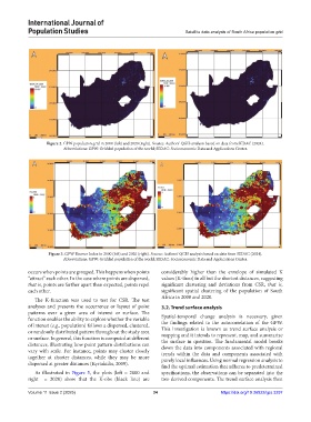
Figure 2. GPW population grid in 2000 (left) and 2020 (right). Source: Authors’ QGIS analysis based on data from SEDAC (2024).
Abbreviations: GPW: Gridded population of the world; SEDAC: Socioeconomic Data and Applications Center.

Figure 3. GPW Hoover Index in 2000 (left) and 2020 (right). Source: Authors’ QGIS analysis based on data from SEDAC (2024).
Abbreviations: GPW: Gridded population of the world; SEDAC: Socioeconomic Data and Applications Center.

occurs when points are grouped. This happens when points considerably higher than the envelope of simulated K
“attract” each other. In the case where points are dispersed, values (K-theo) in all but the shortest distances, suggesting
that is, points are farther apart than expected, points repel significant clustering and deviations from CSR, that is,
each other. significant spatial clustering of the population of South
Africa in 2000 and 2020.
The K-function was used to test for CSR. The test
analyses and presents the occurrence or layout of point 3.2. Trend surface analysis
patterns over a given area of interest or surface. The
function enables the ability to explore whether the variable Spatial-temporal change analysis is necessary, given
of interest (e.g., population) follows a dispersed, clustered, the findings related to the autocorrelation of the GPW.
or randomly distributed pattern throughout the study area This investigation is known as trend surface analysis or
or surface. In general, this function is computed at different mapping and it intends to represent, map, and summarize
the surface in question. The fundamental model breaks
distances, illustrating how point pattern distributions can down the data into components associated with regional
vary with scale. For instance, points may cluster closely trends within the data and components associated with
together at shorter distances, while they may be more purely local influences. Using normal regression analysis to
dispersed at greater distances (Kyriakidis, 2009).
find the optimal estimation that adheres to predetermined
As illustrated in Figure 5, the plots (left = 2000 and specifications, the observations can be separated into the
right = 2020) show that the K-obs (black line) are two derived components. The trend surface analysis then

Volume 11 Issue 2 (2025) 34 https://doi.org/10.36922/ijps.3297