Page 43 - IJPS-11-2

International Journal of
Population Studies Satellite data analysis of South Africa population grid

A B

C D

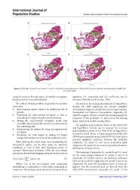
Figure 6. GPW first- (A and B) and second- (C and D) order trend surface function in 2000 and 2020. Source: Authors’ estimates using R-studio (left)
and QGIS (right).
using the structure through space, dictated by variograms, equations, the monomials and (λj) coefficients can be
Kriging method is assumed superior. estimated (Hutchinson & Gessler, 1994).
The ordinary Kriging method, in general, incorporates The results of the Kriging interpolation (in logarithmic
these steps: format) for 2000 employing the Natural Neighbor
• Removing any spatial trend in the underlying data, if Interpolation (Appendix A5 panel A) and average Gaussian,
present. Exponential and Spherical Interpolation (Appendix A5,
• Estimating the experimental variogram, γ, that is, panel B) suggest a further concentration and geographical
calculating the degree of spatial autocorrelation. expansion of the population in and around the existing
• Stating the experimental variogram model that major population centers, among others.
optimally characterizes the spatial autocorrelation in
the underlying data. The population interpolation (based on the 2000 GPW
• Interpolating the surface by using the experimental and logarithmic format) can be assessed for accuracy
variogram. and reliability in terms of the 2020 GPW (in logarithmic
• Producing the final output by adding the kriged format) for South Africa. A visual comparison of the 2000
interpolated surface to the trend interpolated surface. GPW-based interpolation and 2020 GPW for South Africa
revealed significant similarity between the predicted
When plotting the above steps and constructing the (Appendix A5, panel C) and actual population grids
interpolated surface can be done using the statistical (Appendix A5, panel D), in terms of population location,
conditions of “free of bias” and “minimum spread or distribution, density and size.
variance” (Hutchinson & Gessler, 1994), the twin version
can express the universal kriging interpolation function as: The heatmaps (Appendix A5, panels E and F), based
on the raster images displayed in panels C and D of
F ()r = T ()r + ∑ N j= 1 λ jC (r rj− ) (V) Appendix A5, further support the similarity inference
between the predicted (Appendix A5, panel C) and actual
Where T(r) is the non-random drift component (Appendix A5, panel D) population grids. It, however,
representing a combination of low-order monomials in appears that the predicted grid (as derived from the
linear form. By solving a combination of simulations linear 2000 GPW interpolation, Appendix A5, panel E) has

Volume 11 Issue 2 (2025) 37 https://doi.org/10.36922/ijps.3297