Page 15 - IJPS-3-2

Heuveline P and Hong S

To further control for parental characteristics (literacy, occupation, land/craft-tool ownership), we limited the next
analyses to children residing with at least one parent. Table 2 also presents estimates of the odds of school enrollment
controlling for maternal characteristics for children residing with their biological mother, with or without a co-resident
biological father; and similar estimates controlling for paternal characteristics for children residing with their biological
father, with or without a co-resident biological mother. Controlling for maternal characteristics, the odds ratio of school
enrollment for children residing without their biological father is slightly reduced compared to children residing with
their biological father—from 0.66 to 0.60, difference still significant at the 10% level only. For children residing with
their biological father, the odds ratio of school enrollment for children residing without relative to children residing
with their biological mother is even lower (0.56, but the difference is not significant due to the small number of children
not living with their mother). The estimated odds ratios corresponding to household structures other than nuclear or
multi-generational remain largely unchanged by the addition of parental characteristics in the model (from 1.69 for all
children to 1.59 for children living with their mother and 1.71 for children living with their father). Among the parental
characteristics accounted for in these models, literacy and non-farming occupations have strong positive association with
children’s school attendance. Children whose parents are employed in farming are less likely to be in school, especially if
their parents are paid laborers, rather than land owners or tenants. Also notable across models is the absence of significant
gender differences in school attendance.

3.2 Grade for Age
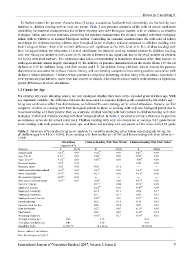
For children who were attending school, we next examined whether they were at the expected grade for their age. With
our dependent variable—the difference between the actual and the expected highest grade completed by the child’s age—
being now continuous rather than dichotomous, we followed the same strategy as for school attendance. Namely, we first
compared children co-residing with both biological parents to those co-residing with only one biological parent and to
those not residing with their parents; then we compared children residing with both parents to children residing with their
biological mother and children residing with their biological father. In Table 3, we observe similar differences by parental
co-residency as we do for school enrollment. Children residing with only one parent are on average 0.23 grade below
those residing with both parents at the same age, and those not residing with any parent a little lower still (0.28 grade

Table 3. Summary of hierarchical regression analysis for variables predicting actual minus expected grade for age for
all children aged 6 to 14 (n = 9,399), those residing with their mother (n = 8,705) and those residing with their father (n =
7,863)
All Children Children Residing With Their Mother Children Residing With Their Father
(Ages 6 to 17)
Predictor B SE(B) B SE(B) B SE(B)
Female child 0.23 ** 0.03 0.23 ** 0.03 0.25 ** 0.03
Ages 9 to 11 -1.01 ** 0.03 -1.00 ** 0.03 -0.98 ** 0.03
Ages 12 to 14 -1.92 ** 0.03 -1.88 ** 0.03 -1.86 ** 0.03
Deceased mother 0.27 † 0.12 -- -- 0.28 0.29
Deceased father 0.02 0.08 -0.07 0.10 -- --
Multi-generational household 0.16 ** 0.05 0.13 * 0.05 0.12 † 0.05
Other households 0.25 ** 0.05 0.13 * 0.05 0.12 † 0.05
No co-resident parent -0.28 ** 0.08 -- -- -- --
Only one co-resident parent -0.23 ** 0.07 -0.24 * 0.08 -0.53 † 0.26
Parent is: Literate 0.73 ** 0.04 0.70 ** 0.05
Employed in crafts 0.72 ** 0.05 0.44 ** 0.09
Employed in industry -0.10 0.19 0.00 0.17
Employed in services 0.11 0.17 0.09 0.15
Employed in civil service 0.83 ** 0.21 0.57 ** 0.16
Sector unknown -0.05 0.18 -0.18 0.18
Parent is: User for free -0.00 0.14 0.03 0.15
User for fee/rent -0.23 * 0.07 -0.15 † 0.07
Paid laborer -0.02 0.07 -0.39 ** 0.12
Ownership unknown 0.38 † 0.17 0.33 † 0.15
Hh level variance (ψ) 0.94 0.73 0.74
Intra-class correlation (ρ) 0.45 0.40 0.40
Model fit (-2LL) 16,289.57 14,678.69 13,238.50
Source: Authors’ calculations.
Note: See footnote to Table 2.

International Journal of Population Studies | 2017, Volume 3, Issue 2 9