Page 49 - IJPS-8-2

International Journal of
Population Studies Used versus Offered densities of human population

easy to visualize that the area below the PDF curve amounts
to 1. The CDF functions are easier to depict jointly than
their PDF counterparts. Using conventional abscissas
(Figure 5B), function F increases in a smooth way paved
U
by the decile values, while function F increases in a one-
O
shot way at low values of x, making the decile values hardly
legible. The recourse to log-scale on the x-axis (Figure 5C)
enables one to visualize the magnitude of the deciles. The
graphical practicality of density magnitudes, that is, of the
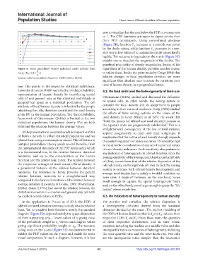
Figure 8. Stair’s generalized density indicators under reduced form logarithms of the human density, provides another reason
ln(x k r / M O )/(k + 1 2 ) r to utilize them, beside the point made by Craig (1984) that
Source: author’s calculations based on INSEE (2021a; 2021b) relative changes in local population densities are more
significant than absolute ones to assess the variations over
one: This points to the respective statistical individuals. time of human density in a geographical space.
Lewontin & Levins (1989) went further in the probabilistic 4.2. On land units and the heterogeneity of land-use
representation of human density by considering spatial
cells of unit ground area as the statistical individuals in Ottensmann (2018a) studied and discussed the definition
geographical space as a statistical population: The cell of spatial cells, in other words, the zoning system to
attribute of local human density is inherited by the people consider for local density and its assignment to people
inhabiting the cells, therefore constituted the used density according to their zones of residence. Craig (1984) studied
as an RV in the human population. Yet, the probabilistic the effects of three zoning systems on the values of the
framework of Ottensmann (2018a) is limited to the two used density in Great Britain as of 1971: He stated that
statistical populations, the human density RVs on both “both the means (of offered and used density) increase as
sides and the relations between the average values. the (spatial) units are progressively subdivided.” This is a
straightforward consequence of the law of total variance
In the present article, we introduced the respective PDFs applied progressively to finer and finer subgroups. It
of human density in either statistical population and we emphasizes that the notion of used density strongly depends
related them using a consumption model. This affiliation to the underlying system of residence zones. This must be kept
(simple) probabilistic theory yields several benefits, from in mind in the consideration of any set of numerical values
the mathematical statement of the PDF relationship which of used density indicators. Such sensitivity also pertains to
is a fundamental one, to the relation between statistical any indicator of heterogeneity in offered densities, since the
moments, and up to the consideration of the Lorenz zoning sensitivity of the average used density, on the left side
function and the related Gini index. The relation between of (16a), comes from that of the relative dispersion of the
the respective averages of used versus offered density is offered density, on the right side of (16a). In fact, the zoning
a prominent instance of the relation between statistical system to estimate both offered density heterogeneity and
moments. The reference to theory provides the general average used density has to satisfy a twofold condition on
relation between moments in a straightforward way, zone sizes: A trade-off between, on the one hand, zones
compared to the former derivations of the relation between small enough to capture the spatial heterogeneity finely
average densities (Lewontin & Levins, 1989; Ottensmann, and, on the other hand, zones large enough to grasp the “life
2018a). Stairs (1977a) had stated the relation between the basins” where people live.
statistical moments in a concise and general way, yet with
no explicit consideration of PDFs. 4.3. On indicators of heterogeneity in human density
In the application to France as of 2019, the PDFs of For positive real variables, the relative dispersion is
offered and used densities were easy to study on a standalone a heterogeneity indicator derived from the standard
basis. Yet, to visualize both functions jointly, the standard deviation divided by the mean. The explicit modeling of
diagram (Figure 5D) depicted mainly the quasi-disjunction the PDFs of human densities, that is, f and f , induces their
U
o
of their supporting sets – lower values of x giving most respective CDFs f and f : From these stem, the quantiles
U
o
of the probability weight to x versus much higher values of their respective distribution, and in turn robust
o
giving significant probability weight to x . The recourse statistics, including the median as a middle value and also
U
to log-scale on the x-axis (Figure 5E) was instrumental to interquartile ratios as measures of heterogeneity, including
exhibit the PDF values on the y-axis and enable for some the inter-quartile ratio and the inter-decile one. Not only
visual comparison. In such a diagram, however, it is less are the interquartile ratios simpler than the alternative
Volume 8 Issue 2 (2022) 43 https://doi.org/10.36922/ijps.v8i2.297