Page 46 - IJPS-8-2

International Journal of
Population Studies Used versus Offered densities of human population

1
E lnx 2 ln( 1 2 ) . Therefore, the related geometric is distributed evenly in its area. Of course, this is only an

O
mean  x satisfies the following equalities which makes it a approximation as large communes (meaning communes of
large area) are likely to exhibit significant intra-communal
geometric midpoint between x and x : heterogeneity of human settlement. Based on this assumption,
O
U
1 x we ranked the communes of increasing average density.
2
 x exp( m s ) x exp s 2 x O 1 2 U
O
2 1 2 According to the ranking, we calculated two cumulated
variables: First the land area, second the population. By
dividing the cumulated area up to commune z by the total
(24)
country area, the F CDF is obtained at point x . Similarly, by
o
z
Thus, based on the case of log-normal distributions, it dividing the cumulated population up to commune z by the
may be conjectured that alternative indicators of average total country area, the F CDF is obtained at point x .
density do not yield much gain beyond considering the u z
The next step is to draw the diagram of F versus F , that is,
(xx U ) pair of average densities. the Lorenz curve (Figure 5A). The Gini index is easy to calculate,
,
u
o
O
O
3. A case study of France as of 2019 by accumulating 2 F x .( F x z 1 )
F x
F x
z
O
O
z
U
z
3.1. The territory under study over communes z. The outcome is 0.76, again a very large value.
Furthermore, easy to calculate are the mean value, variance,
Metropolitan France comprises about 34,750 municipalities standard deviation, and relative dispersion of the density
called “communes” (INSEE, 2021a). We take them as zones variable either offered or used. The results are, in persons per
in the country. The country area of about 543 thousand square kilometer:
square km yields an average commune area of 15.6 km²
(Aliaga et al., 2015). • for x : E x 120 and SD x 548 , yielding
O O O
As of 2019, the French metropolitan population 458. (dimensionless).
O
amounts to about 65 M inhabitants (INSEE, 2021b).
Thus, the average commune population is 1800 people • for x : E x 2 628, and SD x 4 691, , yielding
U
U
U
only and the overall spatial density of population is about 1.79 (dimensionless).
120 persons per km². Figure 4 exhibits the map of French U
communes colored according to density level in the way of Figure 5B and C depicts the empirical CDFs F and F ,
U
O
either the INSEE (Aliaga et al., 2015), the French National together with log-normal approximations that mimic the
Institute for Economic Statistics, or Eurostat, the statistical mean and variance of each distribution. To obtain PDFs
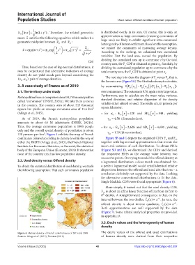
body of the European Union (Eurostat, 2019). It shows that (Figure 5D and E), we discretized the CDFs and derived
most of the country area has low population density. the respective PDFs as the average value between two
successive points. On trying to model the offered density as
3.2. Used density versus Offered density a lognormal distribution, a close match was obtained: Yet,
To obtain the statistical distribution of used density, we made a perfect lognormal model would entail identical relative
the following assumption: That each commune’s population dispersions between the offered and used distributions – a
conclusion definitely not supported by the data. Looking
for alternative conventional distributions to fit the data,
Singh-Maddala CDFs were found appropriate (Figure 6).
More simply, it turned out that the used density CDF,
F , is about an affine linear function of Inx from its first to
U
8 deciles. A straightforward consequence is that, on the
th
1
interval between the two deciles, f ˘ U ()x x . In turn, the
2
offered density is about inverse quadratic, f ˘ O ()x x .
Both approximations are well supported by the data
(Figure 7). Some related analytical properties are provided
in appendix D.
3.3. Decile values and the heterogeneity of human
density
Figure 4. Human density of French communes as of 2015 and 2018 The decile values of the offered and used distributions
Sources: Aliaga et al. (2015), Eurostat (2019) of human density were derived from their respective
Volume 8 Issue 2 (2022) 40 https://doi.org/10.36922/ijps.v8i2.297