Page 44 - IJPS-8-2

International Journal of
Population Studies Used versus Offered densities of human population

A B

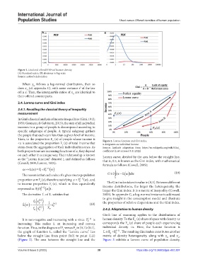
Figure 1. Used and offered PDFs of human density
(A) Standard scales, (B) abscissas in log-scale
Source: author’s elaboration

When x follows a log-normal distribution, then so
O
does x (cf. appendix C), with same variance s of the law
2
U
of ln x: Then, the interquartile ratios of x are identical to
U
their offered counterparts.
2.4. Lorenz curve and Gini index
2.4.1. Recalling the classical theory of inequality
measurement
In Gini’s classical analysis of income inequalities (Gini, 1912;
1955; Gionanni & Gubbiotti, 2015), the sum of all individual
incomes in a group of people is decomposed according to
specific subgroups of people. A typical subgroup gathers
the people that each earn less than a given level of income.
Then, to the proportion F (x) of-people whose income is Figure 2. Lorenz function and Gini index
P
<x is associated the proportion F (x) of total income that x designates an individual income
I
stems from the aggregation of their individual incomes. As Source: Author’s adaptation from https://en.wikipedia.org/wiki/Gini_
both proportions are increasing functions of x, they depend coefficient [Last accessed 8.11.2022]
on each other in a unique way. Their relationship is known Lorenz curve, divided by the area below the straight line,
as the “Lorenz function” denoted L and defined as follows that is, 0.5, is known as the Gini index, with mathematical
(Cowell, 2009; Lorenz, 1905): formula as follows (Cowell, 2009):

L() F I F P (1 ) 1

The reason is that each value of x gives rise to population G 2 ( )L d (19)
0
proportion α ≡ F (x), therefore satisfying x F P ( 1 ) () , and
I
to income proportion F (x), which is thus equivalently The Gini index takes its value in [0,1]. Between different
I
1

expressed as FF( P . income distributions, the larger the heterogeneity, the
)
larger the Gini index: It is a metric of inequality (Cowell,
I

The derivative L of L satisfies that 2009). In appendix C, a log-normal instance is addressed
I
f x p 1 to give insight in the consumption model and illustrate
the properties of relative dispersions and the Gini index.

L x P (18)
P
f x p x P 2.4.2. Adaptation to human density
Gini’s line of reasoning applies to the distributions of
It is non-negative and increasing with α since F P (−1 ) is human density: To the F (x) share of space with density <x
O
increasing: This makes L an increasing and convex corresponds the F (x) share of people each experiencing
U
function. Thus, in the diagram of F versus F in [0,1]×[0.1], individual density <x. Here, the Lorenz function is
p
1
the graph of function L, called the “Lorenz curve,” lies LF U  F O ( 1 ) . The resulting Gini index constitutes another
below the straight line from point (0,0) to point (1,1) metric of density heterogeneity, along with γ and γ .
U
O
(Figure 2). The area between the straight line and the Figure 3 exhibits a Lorenz curve of population density,
Volume 8 Issue 2 (2022) 38 https://doi.org/10.36922/ijps.v8i2.297