Page 119 - MI-2-3

Microbes & Immunity Statistical modeling of COVID-19 trends

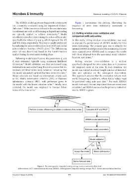
The ARIMA modeling process began with a stationarity Figure 1 summarizes this process, illustrating the
test, commonly conducted using the augmented Dickey– sequence of steps from stationarity assessment to
11
Fuller test. If the time series is found to be non-stationary, forecasting.
transformations such as differencing or logarithmic scaling
are typically applied to achieve stationarity. Model 3.2. Rolling window cross-validation and
10
identification involved determining the orders of the model, comparison with auto.arima
specifically the values of p and q, which represent the AR In this study, rolling window cross-validation was used
and MA terms, respectively. This step is usually performed to evaluate the performance of ARIMA models for time
by analyzing the autocorrelation function (ACF) and partial series forecasting. The primary goal was to identify the
autocorrelation function (PACF) plots. The differencing optimal ARIMA model parameters by minimizing the root
9
order (d) was determined based on the transformations mean squared error (RMSE) and to compare the results
applied during the stationarity testing phase. with those obtained from the automated model selection
Following model identification, the parameters ϕ and function, auto.arima. 14
i
θ were estimated, typically using maximum likelihood Rolling window cross-validation is a method
j
estimation. Model validation was then performed using specifically designed for time series data as it preserves
10
statistical tests such as the Ljung-Box test to ensure that the the temporal order of the data. In each iteration, the
residuals exhibited white noise behavior, indicating that model was trained on a fixed-length window of historical
the model adequately captured the time series structure. data and validated on the subsequent observation.
12
Model selection was based on information criteria such This approach ensures that the evaluation reflects real-
as the Akaike information criterion (AIC) or Bayesian world forecasting conditions, where future values must
information criterion (BIC), with preference given to be predicted using only past data. For each ARIMA
15
13
the model with the lowest criterion value. Finally, once model evaluated, the one-step-ahead forecast errors were
validated, the model was employed to forecast future calculated, and RMSE was used as the primary evaluation
values of the time series. 9 metric. RMSE is given:

Figure 1. The autoregressive integrated moving average model construction flow chart
Abbreviations: ACF: Autocorrelation function; ARIMA: Autoregressive integrated moving average; PACF: Partial autocorrelation function.

Volume 2 Issue 3 (2025) 111 doi: 10.36922/MI025040007