Page 123 - MI-2-3

Microbes & Immunity Statistical modeling of COVID-19 trends

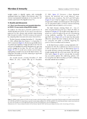
weights matrix to identify regions with statistically 27, 2020. Figure 2D illustrates a closer alignment
significant clustering of high or low infection rates. The between the predicted and actual observed cases,
36
detailed mathematical formulation of the Getis-Ord Gi* with only minor deviations. The ACF and PACF plots
statistic is provided in the Supplementary File. (Figure 2E and F) further support the model’s adequacy,
though some residual correlations persist. The Ljung-Box
4. Results and discussion test for this period yields a p=0.6327, further indicating
4.1. Short-term forecasting and anomaly detection that residual autocorrelation is not a concern.
in COVID-19 case counts using ARIMA models The third forecast, covering March 28 – June 27,
To evaluate the short-term predictive performance of 2021, was generated using data up to March 28, 2021. As
ARIMA models on COVID-19 case counts, forecasts were illustrated in Figure 2G, the model closely aligns with the
generated for four distinct time periods using training actual case counts throughout the period, demonstrating
data from prior months. Predictive accuracy was assessed strong predictive capability. The corresponding ACF
by comparing these forecasts with actual observed data. and PACF plots (Figure 2H and I) show that the model
The first forecast, covering September 27 – December effectively captures the data’s temporal structure, though
27, 2020, utilized data from January 5 to September 27, the Ljung-Box test yields a p=0.0728, suggesting the
2020. As shown in Figure 2A, the forecast generally follows presence of minor residual autocorrelation.
the actual case trajectory, though deviations near the end In the final forecast period, covering September 26 –
of the period highlight the model’s limitations in capturing December 26, 2021, the model included data from January
sudden changes in the data. The ACF and PACF plots 3, 2021, to September 26, 2021. As illustrated in Figure 2J,
(Figure 2B and C) reveal some residual autocorrelation, the model maintains strong performance, with forecasts
highlighting potential areas for model improvement. The closely aligning with the actual case counts. The ACF and
Ljung-Box test yields a p=0.3746, indicating no significant PACF plots (Figure 2K and L) indicate that the model
residual autocorrelation. has successfully captured the underlying patterns, with
The second forecast, covering December 27, 2020 the Ljung-Box test demonstrating a p=0.2876, indicating
– March 28, 2021, utilized data up to December minimal residual autocorrelation.

A B C

D E F

G H I

J K L

Figure 2. ARIMA model analysis of COVID-19 case forecasts in the United States across four time periods. First forecast period: Actual versus predicted
(A), ACF (B) and PACF (C); second forecast period: Actual versus predicted (D), ACF (E) and PACF (F); third forecast period: Actual versus predicted
(G), ACF (H) and PACF (I); and fourth forecast period: Actual versus predicted (J), ACF (K) and PACF (L).
Abbreviations: ACF: Autocorrelation function; CI: Confidence interval; PACF: Partial autocorrelation function; USA: United States of America.

Volume 2 Issue 3 (2025) 115 doi: 10.36922/MI025040007