Page 53 - MSAM-2-1

Materials Science in Additive Manufacturing Data imputation strategies of PBF Ti64

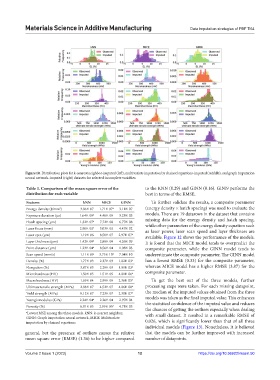
Figure 10. Distribution plots for k-nearest neighbor-imputed (left), multivariate imputation by chained equations-imputed (middle), and graph imputation
neural network-imputed (right) datasets for selected incomplete variables.

Table 3. Comparison of the mean square error of the to the KNN (0.29) and GINN (0.16). GINN performs the
distribution for each variable best in terms of the RMSE.
Features kNN MICE GINN To further validate the results, a composite parameter
Energy density (J/mm ) 3.06E-07 1.71E-07 a 3.11E-07 (energy density × hatch spacing) was used to evaluate the
3
Exposure duration (µs) 1.64E-05 a 4.46E-05 3.23E-05 models. There are 19 datarows in the dataset that contains
Hatch spacing (µm) 1.32E-07 a 7.72E-08 6.77E-08 missing data for the energy density and hatch spacing,
Laser focus (mm) 2.90E-02 a 3.03E-02 4.47E-02 while other parameters of the energy density equation such
as laser power, laser scan speed and layer thickness are
Laser spot (µm) 1.19E-06 8.50E-07 2.97E-07 a available. Figure 12 shows the performance of the models.
Layer thickness (µm) 1.42E-09 a 2.88E-09 4.26E-09 It is found that the MICE model tends to overpredict the
Point distance (µm) 1.23E-04 a 8.56E-04 1.03E-03 composite parameter, while the GINN model tends to
Scan speed (mm/s) 1.11E-09 3.75E-10 a 7.04E-10 underestimate the composite parameter. The GINN model
Density (%) 1.77E-03 2.27E-03 1.82E-03 a has a lowest RMSE (0.33) for the composite parameter,
Elongation (%) 3.87E-03 2.29E-03 1.81E-03 a whereas MICE model has a higher RMSE (3.87) for the
Microhardness (HV) 1.50E-05 1.51E-05 4.81E-06 a composite parameter.
Macrohardness (HV) 1.69E-04 2.99E-05 2.36E-05 a To get the best out of the three models, further
Ultimate tensile strength (MPa) 2.08E-07 4.52E-07 4.86E-08 a processing steps were taken. For each missing datapoint,
Yield strength (MPa) 9.12E-07 7.23E-07 2.30E-07 a the median of the imputed values obtained from the three
Young’s modulus (GPa) 2.24E-04 a 2.26E-04 2.97E-04 models was taken as the final imputed value. This enhances
the statistical confidence of the imputed value and reduces
Porosity (%) 6.01E-05 2.99E-05 a 4.71E-05 the chances of getting the outliers especially when dealing
a Lowest MSE among the three models. kNN: k-nearest neighbor, with small dataset. It resulted in a remarkable RMSE of
GINN: Graph imputation neural network, MICE: Multivariate
imputation by chained equations 0.026, which is significantly lower than that of all three
individual models (Figure 13). Nonetheless, it is believed
general, but the presence of outliers causes the relative that the models can be further improved with increased
mean square error (RMSE) (1.36) to be higher compared number of datapoints.

Volume 2 Issue 1 (2023) 12 https://doi.org/10.36922/msam.50