
Page 51 - MSAM-4-3
P. 51
Materials Science in Additive Manufacturing AI-driven defect detection in metal AM
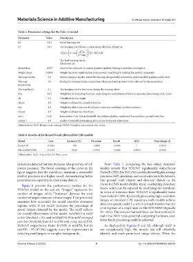
Table 5. Parameter settings for the Yolo‑v5 model
Parameter Value Description
lr0 0.01 Initial learning rate
lrf 0.01 The learning rate follows a cosine decay schedule, defined as:
x *π
lr x () = 1 cos (1 − lrf ) + lrf
*
−
2 * step
The final learning rate is:
lrfinal=lr0+lrf
Momentum 0.937 Used in the optimizer to control gradient updates, helping to stabilize convergence
Weight decay 0.0005 Weight decay for regularization helps prevent overfitting by limiting the model’s complexity
Warmup epochs 3.0 Several warmup epochs, where the learning rate gradually increases to avoid unstable gradients at the start
Warmup 0.8 During the warmup phase, momentum values gradually increase to the value set by the momentum
momentum
Warmup bias lr 0.1 The learning rate for bias terms during the warmup phase
Box 0.05 Weight for the bounding box loss, controlling the contribution of the box regression loss (using CIOU Loss)
cls 0.5 Classification loss weight
cls pw 1.0 Weight coefficient for classification loss
obj 1.0 Weight for object loss uses BCE Loss to measure confidence in object presence
obj pw 1.0 Weight coefficient for object loss
you t 0.25 Intersection Over Union threshold; this defines whether a predicted box matches a ground truth box
anchor t 4.0 Anchor threshold, determining if an anchor box needs adjustment
Abbreviations: BCE: Binary cross-entropy; CIOU: Complete intersection over union.
Table 6. Results of the Resnet50 and EfficientNetV2B0 models
Model Loss Accuracy (%) Precision Recall AUC Time/image (s)
Resnet-50 0.9916 100 1.0000 1.0000 1 0.0272
EfficientNetV2B0 0.0475 99.62 0.9912 1.0000 0.9937 0.0182
Abbreviation: AUC: Area under the ROC curve.
defects are detected but also increases false positives, which From Table 7, comparing the two object detection
lowers precision. The broad coverage of the curve in the models reveals that YOLOv5 significantly outperforms
figure suggests that the model can maintain a reasonable Faster R-CNN. The YOLOv5 model achieved higher average
level of precision at a higher recall, demonstrating better precision (AP), precision, and recall rates on both datasets.
generalization capability in identifying defects. The ground truth objects and detected objects in the
Figure 8 presents the performance metrics for the Faster R-CNN model display many overlapping detection
YOLOv5 model on the test set. “Images” represents the boxes, which can be adjusted by modifying the threshold.
number of images, while “Instances” denotes the total In terms of inference time, YOLOv5 is significantly faster
number of target instances in those images. P (or precision) than Faster R-CNN. By directly processing high-resolution
measures how accurately the model identifies abnormal images on standard CPU resources, both models achieve
regions, while R (or recall) indicates the percentage of detection speeds under 2 s, which is much shorter than the
actual defects detected by the model. The mAP reflects printing time of a single layer on the EOS M290 (typically
the overall effectiveness of the model. mAP@0.5 is mAP 10 – 60 s). This ensures that each layer can be monitored in
at IoU threshold = 0.5, and mAP@0.5:0.95 is mAP averaged real-time. With more powerful computing hardware, even
over IoU thresholds from 0.5 to 0.95 with a step size of 0.05. faster batch processing could be achieved.
YOLOv5 outperforms Faster R-CNN at mAP50, but its As displayed in Figures 9 and 10, although mAP is
mAP50 – 95 (47.3%) suggests room for improvement in not exceptionally high, the models can still effectively
detecting small targets or complex backgrounds. identify and mark prominent image defects. When the
Volume 4 Issue 3 (2025) 9 doi: 10.36922/MSAM025150022