Page 251 - AJWEP-22-4

HEC-RAS study of Simike–Nzovwe drainage

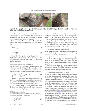
Figure 3. Photographs of the trapezoidal side drain showing (from left to right) the upstream inlet, downstream
outlet, and channel approach section

where the specific energy is minimized. Critical flow Where v is the flow velocity (m/s); n is the Manning’s
occurs when the Froude number (Fr) is equal to 1, roughness coefficient (sm ), R is the hydraulic
-1/3
.
meaning the flow velocity equals the speed of shallow radius (m), which is the cross-sectional area divided
water waves, and is given by Equation II. A Fr <1 by the wetted perimeter (m); and S is the slope of the
indicates subcritical flow (slow, deeper flow) while that energy grade line (water surface slope, m/m).
of more than 1 indicates supercritical flow (fast, shallow Manning’s equation is crucial for calculating flow
flow). depths and velocities, particularly under subcritical
v 2 conditions where frictional forces prevail.
E = + (I)
y
2g
2.2.4. Hydraulic jump and flow transition
v When water transitions from supercritical to subcritical
Fr = (II)
gy flow, a hydraulic jump occurs. The associated energy
loss can be calculated using Equation V.
Where E is the specific energy (m); y is the flow h = y -y (V)
depth (m); v is the velocity of the flow (m/s); g is the L 2 1
acceleration due to gravity (m/s ); and Fr is the Froude Where h is the energy loss during the hydraulic
2
L
number (unitless). jump; y is the downstream water depth after the
2
jump (m); and y is the upstream water depth before the
1
2.2.2. Energy equation for flow profiles jump (m).
The HEC-RAS uses the energy equation to compute The downstream depth (y ) can be estimated from
2
water surface profiles for gradually varied flow, which the upstream depth (y ) using the momentum equation,
1
is critical for understanding how water levels change in typically requiring iterative methods to solve.
roadside drainage systems and is given by Equation III. 2.2.5. Application of the HEC-RAS model
v 1 2 + y + z = v 2 2 + y + z + h (III) To set up the HEC-RAS model, surveyed reduced
2g 1 1 2g 2 2 L levels and cross-sectional geometry data were pre-
Where v , v are the velocities at two different sections processed and imported into the model environment.
1
2
(m/s); y , y are the depths at two different sections (m); All culvert locations along the 1.85 km drainage section
1
2
z , z are the channel bed elevations (m); h is the head were identified and accurately represented within the
2
L
1
loss due to friction and channel resistance (m). model by inputting their respective dimensions and
This equation ensures energy conservation along placements. The elevation data showed a difference
the flow, accounting for frictional losses, which are of 66.969 m between the upstream and downstream
modeled using Manning’s equation. reaches. A longitudinal profile was generated, and cross-
sections were interpolated at 50-m intervals to ensure
2.2.3. Manning’s equation continuity and detail (Figure 4). The simulations were
To compute the open channel flow velocities, Manning’s conducted under steady-state flow conditions with flow
3
3
equation (Equation IV) is utilized. discharges ranging from 3.5 m /s to 7.5 m /s, capturing
both typical and extreme hydraulic scenarios. Boundary
1 2 1
v = × R × 3 S (IV) conditions were defined as a known upstream flow rate
2
n and a normal depth at the downstream end. Manning’s
Volume 22 Issue 4 (2025) 243 doi: 10.36922/AJWEP025190146