Page 101 - AJWEP-v22i3

Advancing molecular property prediction using graph neural networks

3.2. Model architectures of 1.0 indicates a perfect classifier. The GCN, GAT, and
3.2.1. GCN GIN consist of two, two, and three layers, respectively.
GCN aggregates node features from neighbors using There are 64 hidden dimensions. The networks have
the propagation rule in Equation I: a 50% dropout for regularization. Experiments were
conducted on a system with an NVIDIA A100s
1 − 1
−
ˆ
2 ˆ ˆ
( ) l
H ( 1) = σ (D AD H W ( ) l ) (I) graphics processing unit and 16 GB of random-
l+
2
Where A=A+I the adjacency matrix with self-loops access memory. The models were implemented using
PyTorch and PyTorch Geometric libraries. Random
D is the degree matrix, H represents node features at seeds were set for reproducibility, and all results were
(l)
layer l, H is the learnable weight matrix, and σ is the averaged over five runs with different train-test splits.
(l)
activation function. This methodology ensures a rigorous evaluation of the
GNN architectures for molecular property prediction
3.2.2. GIN on the MUTAG dataset. The algorithm for training is
GIN uses a sum-based aggregation to enhance as follows:
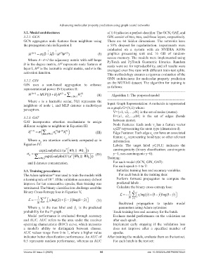
representational power IN Equation II: -------------------------------------------------------------------
( 1)+l = H ((1+ MLP ) H ()l +ò ∑ ∈ j N () i H ()l j (II) Algorithm 1: The proposed model
Where ϵ is a learnable scalar, N(i) represents the ------------------------------------------------------------------
neighbors of node i, and MLP denotes a multi-layer Input: Graph Representation: A molecule is represented
perceptron. as a graph G=(V,E) where:
V={v1, v2,…,vN} is the set of nodes (atoms).
3.2.3. GAT E={e1, e2,…,eM} is the set of edges (bonds
GAT incorporates attention mechanisms to assign between atoms).
different weights to neighbors in Equation III: Node Features: Each node v has a feature vector
i
x ∈R representing the atom type (dimension d).
d
i
()l
h i ( 1)l+ = σ (∑ jòN () i α ()l Wh ()l j ) (III) Edge Features: Each edge e can have an associated
ij
ij
feature e , representing bond type or other relevant
ij
Where α are attention coefficients computed as in information.
ij
Equation IV: Labels: The target label y∈{0,1} indicates the
exp(LeakyReLU (a T    Wh Wh  )) carcinogenicity (binary classification: carcinogenic
α = i j (IV) y=1, non-carcinogenic y=0).
∑ k ∈N ()i exp(LeakyReLU (a T [Wh i  Wh k ] )) Training:
ij
and ∥ denotes concatenation. For each model (GCN, GIN, GAT):
For each epoch t=1 to T:
3.3. Training procedures Initialize training loss and accuracy variables.
The Adam optimizer was used to train the models with For each batch in the training data:
58
a learning rate of 10 . If the validation accuracy did not Perform forward propagation to compute the
−3
improve for ten consecutive epochs, then training was predicted labels .
terminated. The binary classification challenge used the Calculate the binary cross-entropy loss:
Binary Cross-Entropy loss in Equation V, =  − 1 ∑  y log( ) ˆ +y (1− y ) ˆ log(1− ) ˆ  y
N
1 N N = i 1   i
=  − ∑ 1  y log( ˆ) +y (1− y ) ˆ log(1− ˆ) y (V)
N = i  i Backward propagation to update model
Where y is the true label and ˆ y is the predicted parameters using Adam optimizer.
i
i
probability for the i graph. Track training loss and accuracy for the batch.
th
Model performance is evaluated through accuracy Evaluate model performance on the validation set
and AUC. AUC refers to the area under the receiver after each epoch.
operating characteristic (ROC) curve, which measures Implement early stopping if the validation loss
a model’s ability to distinguish between classes. does not improve after a specified number of
AUC values range from 0 to 1, where a higher value epochs.
indicates better classification performance. An AUC of After training the models, evaluate them on the test set.
0.5 represents random performance, whereas an AUC For each batch in the test set:

Volume 22 Issue 3 (2025) 95 doi: 10.36922/AJWEP025070041