Page 46 - EER-2-1

Explora: Environment
and Resource Statistical analysis of climate time series

To verify the consistency of this proposed explanation In Hasselmann’s theory, short-term random noise
with the observations, the author developed a mathematical (atmospheric weather) leads to longer-term variations (red
model (called Z.1) that takes into account the energy spectra at the ocean level). This is mathematically modeled
exchanges between the sun, the troposphere, and the UOS using a first-order autoregressive process, where the next
while integrating the hypothesized interaction between the step y of the long-term variation depends on the previous
t+1
UOS heat and atmospheric temperature. The constants in step y , weighted by the climatic memory m of the ocean,
t
the model were calibrated using the data observed during and is disturbed by short-term variability x : t
the period 1955 – 2022. The Z.1 program is explained and y = m y + x
summarized in Table 7 of the study. We have reproduced t+1 t t
24
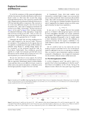
Figure 1 of the study as Figure 2 here. The figure presents In our case, it is the “signals” detected that initially
24
the observed evolutions of the atmospheric temperature guide us: A Markov-1 alternating-type signal is observed
and UOS heat over the period 1955 – 2022, as well as the for both atmospheric (monthly) and oceanic (quarterly)
simulations obtained for these two temperatures over the temperatures. This suggests the presence of an interaction,
period 1955 – 2095, generated by the Z.1 model. and the hypothesis formulated in the Z.1 model posits
Ultimately, the study did not bring anything new for a direct interaction between the two. The difference in
24
MAL itself compared to the previous study. However, periodicity between the two signals is attributed to the
23
the validation of the explanations for the signals obtained vastly different climatic memories of the atmosphere and
through MAL is notably more thorough, and the simulations the ocean.
obtained using Model Z.1 provide strong support for The Z.1 model is built on this interaction and has
the consistency of the proposed hypothesis with the nothing stochastic apart from the fact that we introduced
observations. Furthermore, these simulations, generated random coefficients to take into account natural variability.
quickly on a simple microcomputer, provide fairly precise Thus, our model is more deterministic and less stochastic
information on the medium-term evolution of two of the compared to Hasselmann’s, even though both emphasize
most important parameters of the Earth’s climate. the critical role of climate memory in the framework.

We can also note that on certain aspects, the method
used in the study is reminiscent of Hasselmann’s theory. 3.3. The third application of MAL
29
25
Like our approach, Hasselmann’s theory involves Markov In another subsequent study, the author returns to a
23
chains and takes into account different climatic memories question that he had already addressed in the first study :
of the world ocean and the atmosphere. It, therefore, seems the influence of cloudiness on the climate. Having at his
interesting to precisely compare these two methods. disposal oceanic cloud cover data spanning a long period

Figure 1. Simulations of Z.3 model for deepening. Reproduced from Zeltz .Notes: Red curve: Simulation of anomalies of deepening, Sn (m). For the other
26
curves: The 95% confidence interval is delimited by the upper curve and lower curve. The central blue curve is the theoretical curve (without taking into
account natural variability) of the deepening anomalies.

Figure 2. Simulations of t and θ over the period 1955 – 2095 compared to the observed temperatures of Ta and Θ during the period 1955 – 2022.
n
n
n
n
Copyright © 2024 Author(s). Reproduced from Zeltz . Notes: Red curve: observed atmospheric temperature, Ta ; Purple curve: simulated atmospheric
24
n
temperature, t ; Blue curve: Observed upper ocean layer temperature, Θ ; Green curve: simulated upper ocean layer temperature, θ . n
n
n
Volume 2 Issue 1 (2025) 5 doi: 10.36922/eer.6109