Page 47 - EER-2-1

Explora: Environment
and Resource Statistical analysis of climate time series

– much longer than for those used in 2021 – the author without any further addition to form the Z.2 model.
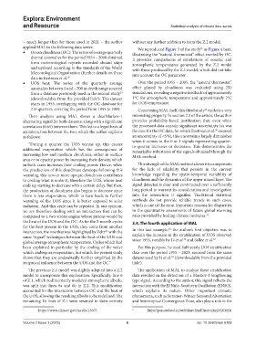
applied MAL to the following data series: We reproduced Figure 3 of the study as Figure 4 here,
25
• Ocean cloudiness (OC): The series of average quarterly illustrating the “natural thermostat” effect exerted by OC.
diurnal anomalies for the period 1954 – 2008 obtained It provides comparisons of simulations of oceanic and
from meteorological reports recorded aboard ships atmospheric temperatures generated by the Z.2 model
and updated according to the standards of the World with those produced by the Z.1 model, which did not take
Meteorological Organization (further details on these into account the OC parameter.
data in Eastman et al. 30
• UOS heat: The series of the quarterly average Over the period 1955 – 2095, the “natural thermostat”
anomalies between 0 and −700 m depth range sourced effect played by cloudiness was evaluated using 250
from a database previously used in the second study simulations, revealing a negative feedback of approximately
24
(downloadable from the provided link ). This dataset 1°C for atmospheric temperature and approximately 2°C
1
starts in 1955, overlapping with the OC database for for UOS temperature.
216 quarters, covering the period from 1955 to 2009. Concerning MAL itself, this third study exploits a very
25
Their analysis using MAL shows a clearMarkov-1 interesting property. In section 2.3 of the article, the author
alternating signal for both datasets, along with a significant provides probability-based justification that, even when
correlation (0.65) between them. This led to a hypothesis of the processed data contain significant uncertainty (as was
30
an interaction between the two, which the author explains the case for the OC data, for which Eastman et al. ensured
as follows: an uncertainty of <5%), this uncertainty largely diminishes
when it comes to the 0 or 1 signals representing quarter-
“During a quarter the UOS warms up, this causes to-quarter increases or decreases. This demonstrates the
additional evaporation which has the consequence of remarkable robustness of the signals obtained through the
increasing low and medium cloudiness, either in surface MAL method.
area or in opacity power by increasing their density, which
in both cases increases their cooling power. Hence, when This strength of the MAL method allows it to compensate
the production of this cloudiness develops following this for the lack of reliability that persists in the current
warming, this new or more opaque cloudiness contributes knowledge regarding the spatio-temporal variability of
to cooling what is under it, therefore the UOS, whose heat cloudiness and the dynamics of the upper mixed layer. The
ends up starting to decrease with a certain delay. But then, signal detected is clear and constructed over a sufficiently
the production of cloudiness also begins to decrease since long period to warrant its consideration and investigation
there is less evaporation, which in turn leads to further into the interaction it signifies. Traditional statistical
warming of the UOS since it is better exposed to solar methods do not provide reliable trends in such cases,
radiation. And this cycle can be repeated. In our opinion, which is one of the most important reasons for disparities
we are therefore dealing with an interaction that can be in the quantitative assessments of future global warming
compared to a two-stroke engine whose pistons would be rates provided by leading climate institutes. 31
the heat of the UOS and the OC. As for the 3-month cycles 3.4. The fourth application of MAL
for the heat present in the UOS, they come from another 26
interaction, the one that was highlighted by Zeltz with the In this last example, the author’s first objective was to
24
same “signal” techniques between the heat of the UOS and explain the increase in the stratification of UOS observed
33
32
global average atmospheric temperature. Cycles which had since 1955, notably by Li et al. and Sallée et al.
been explained in particular by the cooling of the water For this purpose, he used half-yearly UOS stratification
which undergoes evaporation, but which the present study data over the period 1955 – 2023, sourced from the same
shows that they are undoubtedly further amplified by the dataset used by Li et al. (downloadable from the provided
32
reciprocal influence between the UOS and the OC.” link ).
2
The previous Z.1 model was slightly adapted into a Z.2 The application of MAL to analyze these stratification
model to incorporate this explanation. Specifically, line 6 data resulted in the detection of a Markov-1 lengthening
of Z.1, which rudimentarily modeled atmospheric albedo, type signal. According to the author, this signal reflects the
was split into lines 6a and 6b in Z.2. This modification interaction with the El Niño-Southern Oscillation (ENSO),
accounted for the interaction between OC and the heat of which explains its nature. Other important climatic
the UOS, allowing the resulting albedo to be redefined. The phenomena, such as Summer-Winter Seasonal Alternation
remaining 16 lines of Z.1 were retained in their entirety and Intertropical Convergence Zone, also play a role in the

1 https://www.climate.gov/media/13603 2 https://pan.cstcloud.cn/web/share.html?hash=E0zjDQOeRfs

Volume 2 Issue 1 (2025) 6 doi: 10.36922/eer.6109