Page 49 - EER-2-1

Explora: Environment
and Resource Statistical analysis of climate time series

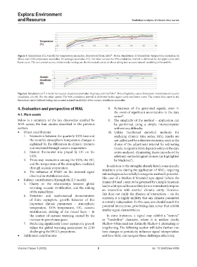
Figure 5. Simulations of Z.3 model for temperature anomalies. Reproduced from Zeltz . Notes: Simulations of atmospheric temperature anomalies, tn
26.
(blue) and UOS temperature anomalies, θn (orange) anomalies (°C). For other curves: the 95% confidence interval is delimited by the upper curve and
lower curve. The two central curves, which nearly overlap, are the theoretical curves (without taking into account natural variability) of tn and θn.

26
Figure 6. Simulations of Z.3 model for oceanic cloudiness anomalies. Reproduced from Zeltz . Notes: Light blue curve: Simulation of anomalies of oceanic
cloudiness, cln (%). For the other curves: The 95% confidence interval is delimited by the upper curve and lower curve. The central blue curve is the
theoretical curve (without taking into account natural variability) of the oceanic cloudiness anomalies.
4. Evaluation and perspective of MAL 8. Robustness of the generated signals, even in
the event of significant uncertainties in the data
4.1. Main assets series .
25
Below is a summary of the key discoveries enabled by 9. The simplicity of the method – application can
MAL across the four studies described in the previous be performed using a simple microcomputer
section: without any difficulty.
• Direct contributions: 10. Unlike traditional statistical methods for
1. Interaction between the quarterly UOS heat and analyzing climatic time series, MAL results are
the monthly atmospheric temperature changes is not influenced by subjective decisions, such as the
explained by the differences in climatic memory choice of the adjustment interval for estimating
and mediated through oceanic evaporation. trends. A signal in MAL depends solely on the data
2. Natural thermostat role played by OC on the series analyzed, eliminating biases introduced by
UOS. arbitrary methodological choices (as highlighted
3. Three-way interaction among the UOS, the OC, by Mudelsee ).
6
and the temperature of the atmosphere mediated In addition to the strengths already listed, some specific
through oceanic evaporation.
4. The influence of ENSO on the detected signal situations arise during the application of MAL, requiring
tailored approaches to fully leverage the method’s potential.
observed in stratification data.
• Indirect contributions (through the Z.3 model): The case of a Markov-0 binomial type signal (where the
5. Clarity on the relationships between global chains of 0 and 1 seem to be governed by a simple binomial
warming, oceanic stratification, and the sinking law) is a bit special because they do not immediately impose
of the mixed layer. an interaction with another climatic entity. However,
6. Detection and mathematical demonstration this does not imply the absence of interactions – on the
of finite asymptotic growth behavior of five contrary, it is highly unlikely that any climatic parameter
important climate parameters – atmospheric is entirely independent. In this case, one should search for
temperature, UOS temperature, OC, oceanic potential interactions, prioritizing data series that exhibit
stratification, sinking of the mixed layer – in similar signal characteristics.
the context of current warming caused by the In some instances, a signal may exhibit a “neutral”
increase in greenhouse gases or “borderline” character, where it is neither clearly
7. Predicting significantly lower asymptotic growth Markov-0 binomial nor distinctly Markov-1 alternating or
values for global warming parameters by 2100 lengthening. The following section will delve further into
challenging the IPCC’s projections. how changes in periodicity influence signal interpretation
• Additional contributions and how MAL can navigate these challenges effectively.

Volume 2 Issue 1 (2025) 8 doi: 10.36922/eer.6109