Page 101 - GHES-1-1

Global Health Econ Sustain Effects of community-based activities on LTC needs

specification of the distribution of the response and (b) the
link function describes how the mean of the response (μ)
j
is linked to a linear combination of the predictors.
For the probit GLM for SAPH, the dependent variable
η is distributed as probit (μ ) is expressed through the
1
1
linear predictor:
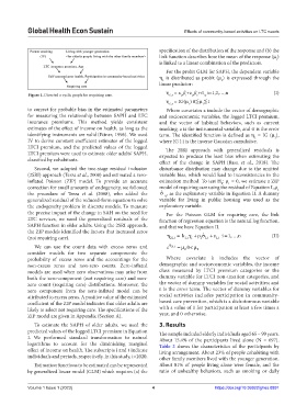
Figure 1. Directed a cyclic graph for requiring care. η = x β +z β +σ i=1,2,…,n (I)
i,t i
i,t
1i,t
i,t z
η = IG(μ ) 0≦μ ≦1
1
1i,t
1
to correct for probable bias in the estimated parameters Where covariates x include the vector of demographic
for measuring the relationship between SAPH and LTC and socioeconomic variables, the logged LTCI premium,
insurance premiums. This method yields consistent and the vector of habitual behaviors, such as current
estimates of the effect of income on health, as long as the smoking. z is the instrumental variable, and σ is the error
identifying instruments are valid (Ettner, 1996). We used term. The identified function is defined as η = IG (μ ),

1
1
.
IV to derive constant coefficient estimates of the logged where IG ( ) is the inverse Gaussian cumulative.
LTCI premium, and the predicted values of the logged The 2SRI approach with generalized residuals is
LTCI premium were used to estimate older adults’ SAPH, expected to produce the least bias when estimating the
classified by cohabitants. effect of the change in SAPH (Basu et al., 2018). The

Second, we adopted the two-stage residual inclusion disturbance distribution may change due to the omitted
(2SRI) approach (Terza et al., 2008) and estimated a zero- variable bias, which would lead to inconsistencies in the
inflated Poisson (ZIP) model. To provide an accurate estimation method. To test H : ρ = 0, we estimate a ZIP
1
0
correction for small amounts of endogeneity, we followed model of requiring care using the residual of Equation I, ρ 1
the procedure of Terza et al. (2008), who added the ˆ σ , as the explanatory variable in Equation II. A dummy
i,t
generalized residual of the reduced-form equation to solve variable for living in public housing was used as the
the endogeneity problem in discrete models. To measure explanatory variable.
the precise impact of the change in SAH on the need for For the Poisson GLM for requiring care, the link
LTC services, we used the generalized residuals of the function of regression equation is the natural log function,
SAPH function in older adults. Using the 2SRI approach, and that we have Equation II.
the ZIP models identified the factors that increased zeros
ˆ σ + ε
(not requiring care). η 2i,t = k γ + ρ 1 i,t i,t i 1,= … ,n (II)
i,t i
We can use the count data with excess zeros and e η 2 it, = µ 0< µ
consider models for two separate components: the 2 2
probability of excess zeros and the accountings for the Where covariate k includes the vector of
non-excess zeros and non-zero counts. Zero-inflated demographic and socioeconomic variables, the income
models are used when zero observations may arise from class measured by LTCI premium categories or the
both the zero-component (not requiring care) and non- dummy variable for LTCI non-taxation categories, and
zero count (requiring care) distributions. Moreover, the the vector of dummy variables for social activities; and
zero component from the zero-inflated model can be ε is the error term. The vector of dummy variables for
attributed to excess zeros. A positive value of the estimated social activities includes participation in community-
coefficient of the ZIP model indicates that older adults are based care prevention, which is a dichotomous variable
likely to select not requiring care. The specifications of the with a value of 1 for participation at least a few times a
ZIP model are given in Appendix (Section A). year, and 0 otherwise.
To estimate the SAPH of older adults, we used the 3. Results
predicted values of the logged LTCI premium in Equation The sample included elderly individuals aged 65 – 99 years.
I. We performed standard transformation to natural About 15.4% of the participants lived alone (N = 697).
logarithms to account for the diminishing marginal Table 2 shows the characteristics of the participants by
effect of income on health. The subscripts i and t indicate living arrangement. About 23% of people cohabiting with
individuals and periods, respectively. In this study, t=2020. other family members lived with the younger generation.
Estimation functions to be estimated can be represented About 81% of people living alone were female, and the
by generalized linear model (GLM) which requires (a) the ratio of unhealthy behaviors, such as smoking or daily

Volume 1 Issue 1 (2023) 4 https://doi.org/10.36922/ghes.0891