Page 323 - IJB-10-2

International Journal of Bioprinting Continuous gradient TPMS bone scaffold

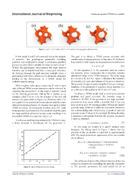
Figure 1. (a) C = 0, G surface; (b) C ≠ 0, G surface; (c) segregation phenomenon.

In this study, G and P cells were utilized as the subjects The goal is to obtain a TPMS porous structure with
of research. The grasshopper parametric modeling continuously changing porosity. In Equation IV, the linear
platform was employed to design a continuous gradient function for C with respect to the parameter z is defined as:
porous structure that is suitable for bone reconstruction. C z (IV)
35
Within the grasshopper environment, the input implicit
function can be transformed into a visual grid structure. In this equation, C is the parameter used to control
By iterating through the grid structure multiple times, a the porosity, while z represents the Z-direction porosity
grid surface with fewer defects can be obtained, ultimately adjustment value of the TPMS structure. The value range
leading to the development of a TPMS model for for z is set to be [0,2.5π]. Figure 2 illustrates the variation
additive manufacturing. of porosity and z per unit volume of the porous structure.
The porosity changes linearly along the Z-axis as z changes.
Within a given cubic space measuring 20 mm on each Similarly, if the parameter C is given a linear function of x
side, different TPMS porous structures can be obtained by or y, the same rule applies to the X-axis or Y-axis.
adjusting the parameter C of the implicit function based
on the existing parameters. Taking the G surface as an To obtain a TPMS model with a continuous porosity
example, when C is set to 0, the porosity of the unit cell gradient and good structure, the porosity range is
remains the same (refer to Figure 1a). However, when C is limited to 30–80%. If the porosity is too high, partition
not equal to 0, the porosity between adjacent units becomes phenomena may occur, while a porosity that is too low
distinct (as shown in Figure 1b). Similar rules apply to other may result in poor 3D printing quality. Within the limited
TPMS structures. Increasing the absolute value of C leads porosity range, different Z values are selected to determine
to an increase in porosity, but if the absolute value becomes the corresponding unit cell porosity. A graph of unit cell
too large, partition phenomena may occur, resulting in an porosity versus Z values is then plotted. By fitting the data,
incomplete TPMS structure (see Figure 1c). a functional relationship between the porosity parameter
C and z is obtained:
To achieve a tunable pore gradient in the TPMS structure,
a linear function is introduced for the parameter C. C 0 1954. z 0 3124. (V)
In this study, six models of G and P surfaces were
designed. The fitting curve in Figure 2 shows that the
porosity of the six models is controlled at approximately
65%. The implicit function expressions of the two models
are as follows:
f(x, y, z) = sin(ωx)cos(ωy) + sin(ωz)cos(ωx)
+ sin(ωy)cos(ωz) = 0.1954*z
+ 0.3124 (VI)

f(x, y, z) = cos(ωx) + cos(ωy) + cos(ωz)
= 0.1954*z + 0.3124 (VII)

The difference between the different models of the two
surfaces is achieved by controlling the periodic parameter
Figure 2. Linear fitting of porosity change ω. The periodic parameters for each model are set as

Volume 10 Issue 2 (2024) 315 doi: 10.36922/ijb.2306