Page 268 - IJB-10-5

International Journal of Bioprinting A TPMS framework for complete dentures

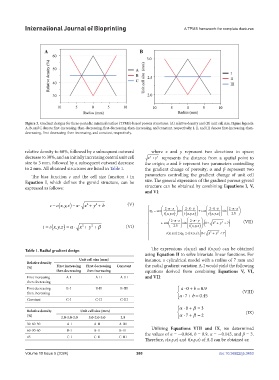
Figure 3. Gradient designs for three-periodic minimal surface (TPMS)-based porous structures: (A) relative density and (B) unit cell size. Figure legends:
A, B, and C denote first-increasing-then-decreasing, first-decreasing-then-increasing, and constant, respectively; I, II, and III denote first-increasing-then-
decreasing, first-decreasing-then-increasing, and constant, respectively.

relative density to 60%, followed by a subsequent outward where x and y represent two directions in space;
decrease to 30%, and an initially increasing central unit cell x + y represents the distance from a spatial point to
2
2
size to 3 mm, followed by a subsequent outward decrease the origin; a and b represent two parameters controlling
to 2 mm. All obtained structures are listed in Table 1. the gradient change of porosity; α and β represent two
The bias function c and the cell size function t in parameters controlling the gradient change of unit cell
Equation I, which defines the gyroid structure, can be size. The general expression of the gradient porous gyroid
expressed as follows: structure can be obtained by combining Equations I, V,
and VI:

c = ( a x + y + b (V) 
c x,y,z) =⋅
2
2
⋅⋅ 
 ϕ = cos  2 π ⋅⋅x  sin  2 π ⋅⋅ y   + cos  π ⋅ 2 ⋅ ⋅ y  sin  2 π z 



G
   ( tx,y,z )     ( tx,y,z )     ( tx,y,z )    25 . 


⋅⋅ 
  + cos  2 π z sin  2⋅⋅ ⋅π y  ( < x 2 + y 2 < 7 ) (VII)
, 0
2
2
t x,y,z) = α
t = ( ⋅ x + y + β (VI)    25 .     ( tx,y,z )  
 ( )
2 2
 −cx,y,z( ) ≤ϕ G ≤ cx,y,z( ), 0 < x + y 2 < 7


Table 1. Radial gradient design The expressions c(x,y,z) and t(x,y,z) can be obtained
using Equation II to solve bivariate linear functions. For
Unit cell size (mm) instance, a cylindrical model with a radius of 7 mm and
Relative density
(%) First increasing First decreasing Constant the radial gradient variation A-I would yield the following
then decreasing then increasing equations derived from combining Equations V, VI,
First increasing A-I A-II A-III and VII:
then decreasing
First decreasing B-I B-II B-III   a ⋅+ =0 b 0.9
then increasing  a ⋅+ = 0.45 (VIII)
b
7
Constant C-I C-II C-III  
  α ⋅+0 β = 3
Relative density Unit cell size (mm)  (IX)
(%) 2.0-3.0-2.0 3.0-2.0-3.0 2.5   α ⋅+7 β = 2
30-60-30 A-I A-II A-III
Utilizing Equations VIII and IX, we determined
60-30-60 B-I B-II B-III the values of a = -0.064, b = 0.9, α = -0.143, and β = 3.
45 C-I C-II C-III
Therefore, c(x,y,z) and t(x,y,z) of A-I can be obtained as:
Volume 10 Issue 5 (2024) 260 doi: 10.36922/ijb.3453