Page 321 - IJB-8-4

Bonatti, et al.
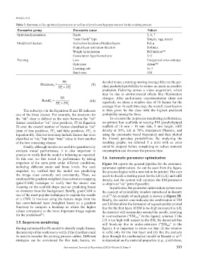
Table 3. Summary of the optimized parameters as well as other relevant hyperparameters for the training process
Parameter group Parameter name Values
Optimized parameters Depth 5, 6, 7
“conv block” type Simple, vgg, resnet
Model architecture Activation function of hidden layers ReLu
Output layer activation function Softmax
Weight initialization HeUniform [45]
Convolution layer kernel size 3×3
Training Loss Categorical cross-entropy
Optimizer Adam [46]
Learning rate 1e-3
Batch size 128

TP decided to use a running moving average filter on the per-
Precision = i (II) class predicted probability to reduce as much as possible
i
TP i + FP i prediction flickering across a video acquisition, which
may be due to environmental effects like illumination
TP changes. After preliminary experimentation (data not
Recall = i (III) reported), we chose a window size of 30 frames for the
i
TP i + FN i average filter. At each time step, the overall classification
The subscript i in the Equations II and III indicates is then given by the class with the highest predicted
one of the three classes. For example, the precision for probability among the three.
the “ok” class is defined as the ratio between the “ok” To evaluate the in-process monitoring performance,
frames classified as “ok” (true positives, TP in Equation we printed four scaffolds at varying EM (parallelepiped
i
II) over the overall number of frames classified as “ok” scaffold of 10 mm × 10 mm side, 5 mm height, infill
(sum of true positives, TP , and false positives, FP , in density at 30%, LH at 70%, transparent Pluronic, and
i
i
Equation III). This last term may include frames that were using the pneumatic-based bioprinter) and then plotted
classified as “ok,” but their “true” value is from another the filtered per-class probabilities. By analyzing the
of the two remaining classes. resulting graphs, we inferred if a print with an error
Finally, although metrics are useful to quantitatively could be stopped before completing to reduce material
evaluate model performance, it is also important in consumption and decrease the process time.
practice to verify that the model is behaving as expected.
To this end, we first tested its performance by taking 3.6. Automatic parameter optimization
snapshots of the same print under different conditions, Figure 3A reports the general pipeline for the automatic
including different zoom and focus levels. For each parameter optimization. As can be seen from the figure,
snapshot, we verified that the model was predicting the process begins with a new ink to be printed. The user
the image class correctly and consistently. Then, we needs to decide a starting point for the LH (LH ) and infill
i
employed the gradient-weighted class activation mapping density, and the system will optimize the EM parameter
(grad-CAM) technique to verify that the model was to obtain an “ok” print if possible.
focusing on the scaffold shape and not predicting based In particular, the parameter optimization system uses
on elements from the background. Briefly, grad-CAM is the concept of printability window introduced in Bonatti
one of the most popular techniques to explain the results et al. An example of such graph is shown in Figure 3B.
[7]
of a CNN. It involves using the feature maps from the Briefly, the central zone indicates the combination of EM
last convolutional layer (weighted based on a gradient and LH that allow the formation of a good-quality printed
function) to compute a heatmap in which the higher line for the first layer. If EM is too high in respect to LH,
values correspond to the most important image regions the material will accumulate around the needle, resulting
for the prediction . in over-extrusion (“EM max” in the figure); whereas if the
[47]
LH is too high with respect to the EM, the deposited line
3.5. In-process monitoring will break-up due to under-extrusion (“EM min” in the
Having optimized the DL model to classify single frames, figure). It is important to stress out that: (i) the window
the next step of the work was to verify if the classifier could is valid only for the first layer and (ii) that the analysis
be used to monitor the printing process online. Different done through the mathematical model in Bonatti et al.
[7]
strategies can be envisioned for this task; herein, we is dependent on the material properties (e.g., yield stress,
International Journal of Bioprinting (2022)–Volume 8, Issue 4 313